Backwards Feature Selection Helper Functions

Ancillary functions for backwards selection

pickSizeBest(x, metric, maximize)

pickSizeTolerance(x, metric, tol = 1.5, maximize)

pickVars(y, size)

caretFuncs

ldaFuncs

treebagFuncs

gamFuncs

rfFuncs

lmFuncs

nbFuncs

lrFuncs

Arguments

x	a matrix or data frame with the performance metric of interest
metric	a character string with the name of the performance metric that should be used to choose the appropriate number of variables
maximize	a logical; should the metric be maximized?
tol	a scalar to denote the acceptable difference in optimal performance (see Details below)
y	a list of data frames with variables Overall and var
size	an integer for the number of variables to retain

Format

An object of class list of length 6.

Details

This page describes the functions that are used in backwards selection (aka recursive feature elimination). The functions described here are passed to the algorithm via the functions argument of rfeControl.

See rfeControl for details on how these functions should be defined.

The 'pick' functions are used to find the appropriate subset size for different situations. pickBest will find the position associated with the numerically best value (see the maximize argument to help define this).

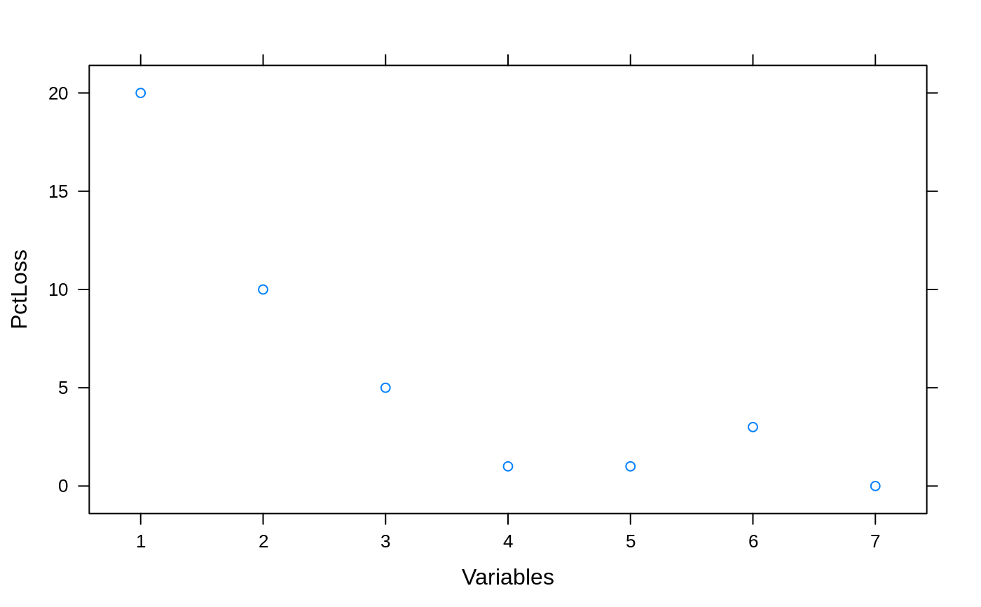
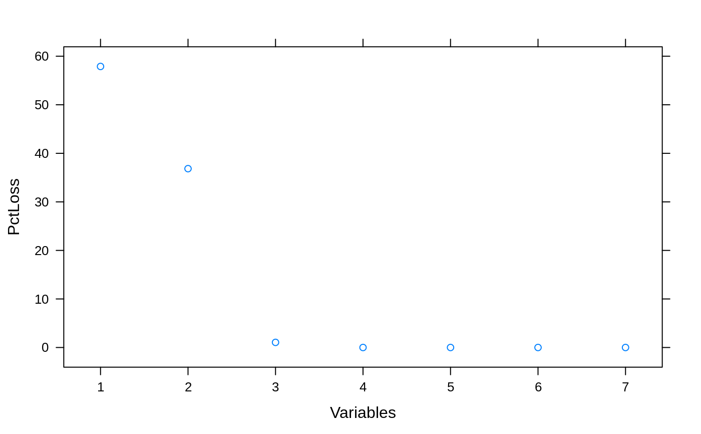
pickSizeTolerance picks the lowest position (i.e. the smallest subset size) that has no more of an X percent loss in performances. When maximizing, it calculates (O-X)/O*100, where X is the set of performance values and O is max(X). This is the percent loss. When X is to be minimized, it uses (X-O)/O*100 (so that values greater than X have a positive "loss"). The function finds the smallest subset size that has a percent loss less than tol.

Both of the 'pick' functions assume that the data are sorted from smallest subset size to largest.

See also

rfeControl, rfe

Examples

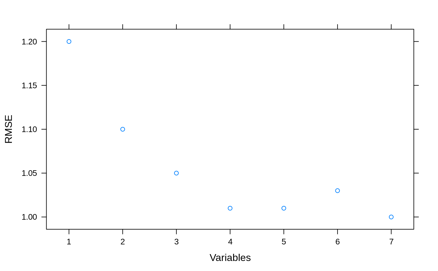
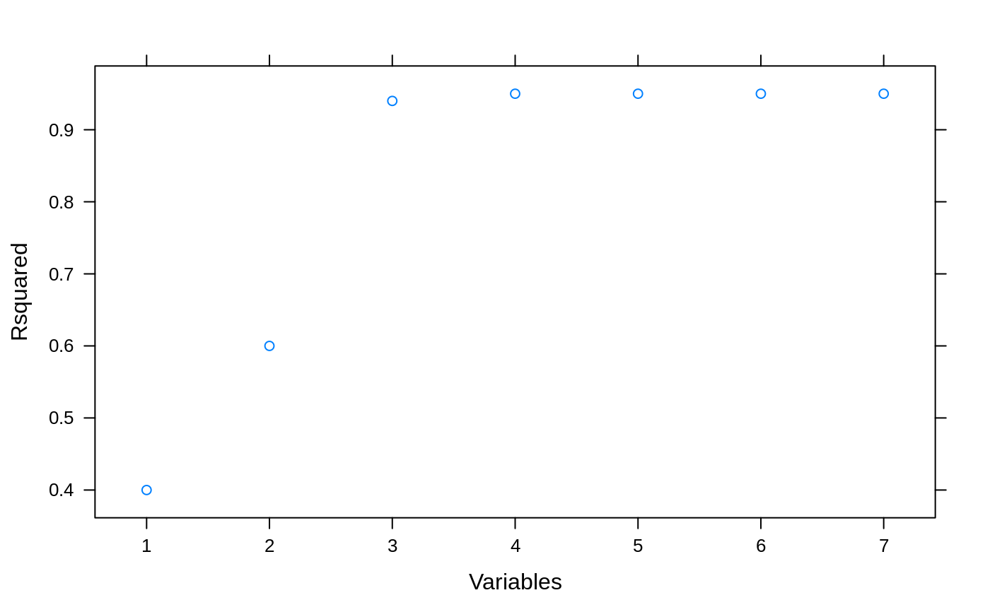
## For picking subset sizes:
## Minimize the RMSE
example <- data.frame(RMSE = c(1.2, 1.1, 1.05, 1.01, 1.01, 1.03, 1.00),
                      Variables = 1:7)
## Percent Loss in performance (positive)
example$PctLoss <- (example$RMSE - min(example$RMSE))/min(example$RMSE)*100

xyplot(RMSE ~ Variables, data= example)
xyplot(PctLoss ~ Variables, data= example)

absoluteBest <- pickSizeBest(example, metric = "RMSE", maximize = FALSE)
within5Pct <- pickSizeTolerance(example, metric = "RMSE", maximize = FALSE)

cat("numerically optimal:",
    example$RMSE[absoluteBest],
    "RMSE in position",
    absoluteBest, "\n")
#> numerically optimal: 1 RMSE in position 7 
cat("Accepting a 1.5 pct loss:",
    example$RMSE[within5Pct],
    "RMSE in position",
    within5Pct, "\n")
#> Accepting a 1.5 pct loss: 1.01 RMSE in position 4 

## Example where we would like to maximize
example2 <- data.frame(Rsquared = c(0.4, 0.6, 0.94, 0.95, 0.95, 0.95, 0.95),
                      Variables = 1:7)
## Percent Loss in performance (positive)
example2$PctLoss <- (max(example2$Rsquared) - example2$Rsquared)/max(example2$Rsquared)*100

xyplot(Rsquared ~ Variables, data= example2)
xyplot(PctLoss ~ Variables, data= example2)

absoluteBest2 <- pickSizeBest(example2, metric = "Rsquared", maximize = TRUE)
within5Pct2 <- pickSizeTolerance(example2, metric = "Rsquared", maximize = TRUE)

cat("numerically optimal:",
    example2$Rsquared[absoluteBest2],
    "R^2 in position",
    absoluteBest2, "\n")
#> numerically optimal: 0.95 R^2 in position 4 
cat("Accepting a 1.5 pct loss:",
    example2$Rsquared[within5Pct2],
    "R^2 in position",
    within5Pct2, "\n")
#> Accepting a 1.5 pct loss: 0.94 R^2 in position 3