Bivariate Data Set with 3 Clusters

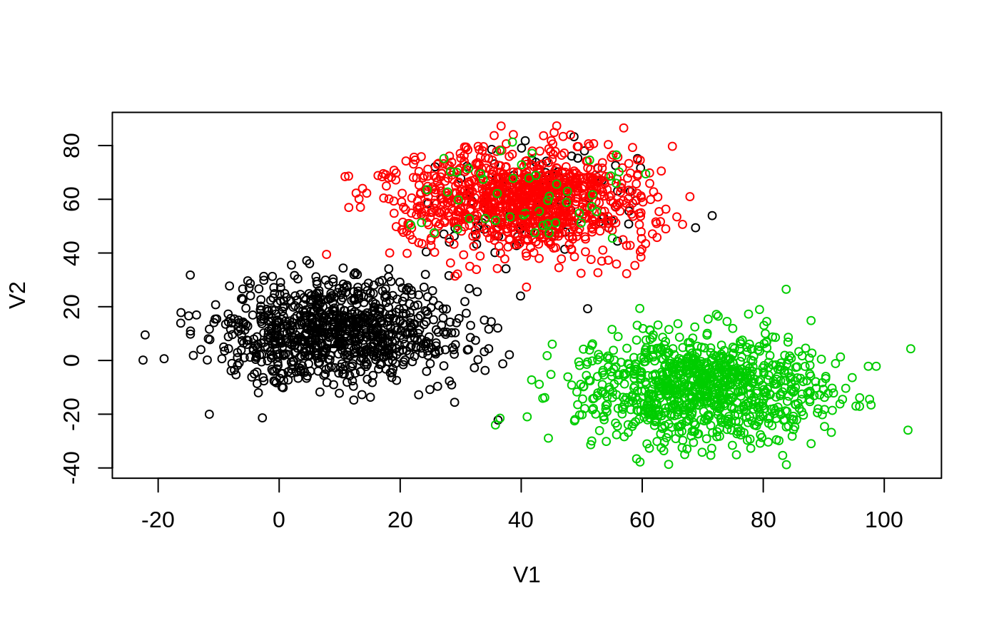
An artificial data set consisting of 3000 points in 3 quite well-separated clusters.

data(xclara)

Format

A data frame with 3000 observations on 2 numeric variables (named V1 and V2) giving the \(x\) and \(y\) coordinates of the points, respectively.

Source

Sample data set accompanying the reference below (file xclara.dat in side clus_examples.tar.gz).

Note

Our version of the xclara is slightly more rounded than the one from read.table("xclara.dat") and the relative difference measured by all.equal is 1.15e-7 for V1 and 1.17e-7 for V2 which suggests that our version has been the result of a options(digits = 7) formatting.

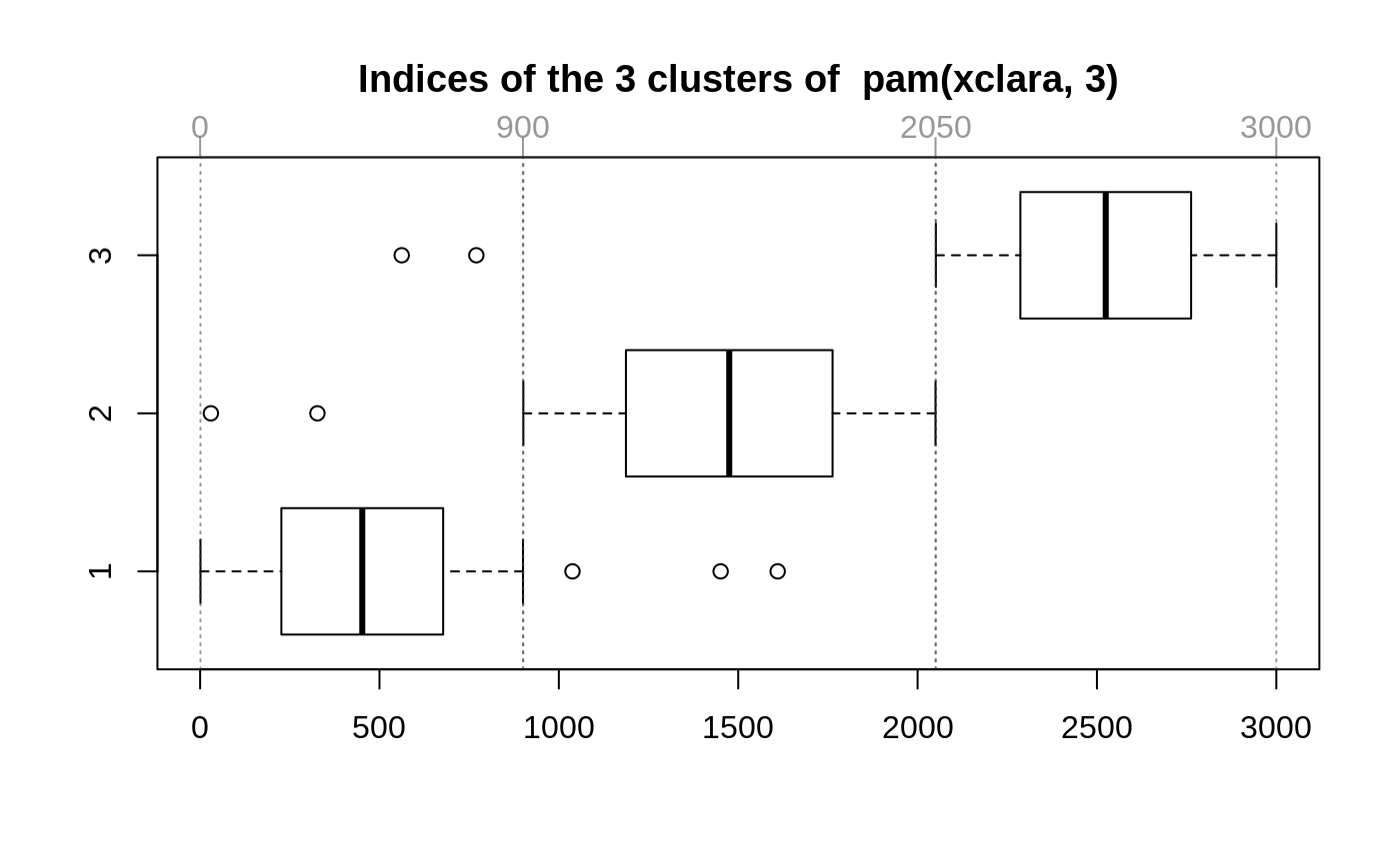
Previously (before May 2017), it was claimed the three cluster were each of size 1000, which is clearly wrong. pam(*, 3) gives cluster sizes of 899, 1149, and 952, which apart from seven “outliers” (or “mislabellings”) correspond to observation indices \(\{1:900\}\), \(\{901:2050\}\), and \(\{2051:3000\}\), see the example.

References

Anja Struyf, Mia Hubert & Peter J. Rousseeuw (1996) Clustering in an Object-Oriented Environment. Journal of Statistical Software 1. doi: 10.18637/jss.v001.i04

Examples

## Visualization: Assuming groups are defined as {1:1000}, {1001:2000}, {2001:3000}
plot(xclara, cex = 3/4, col = rep(1:3, each=1000))
p.ID <- c(78, 1411, 2535) ## PAM's medoid indices  == pam(xclara, 3)$id.med
text(xclara[p.ID,], labels = 1:3, cex=2, col=1:3)

 px <- pam(xclara, 3) ## takes ~2 seconds
 cxcl <- px$clustering ; iCl <- split(seq_along(cxcl), cxcl)
 boxplot(iCl, range = 0.7, horizontal=TRUE,
         main = "Indices of the 3 clusters of  pam(xclara, 3)")

 ## Look more closely now:
 bxCl <- boxplot(iCl, range = 0.7, plot=FALSE)
 ## We see 3 + 2 + 2 = 7  clear "outlier"s  or "wrong group" observations:
 with(bxCl, rbind(out, group))
#>       [,1] [,2] [,3] [,4] [,5] [,6] [,7]
#> out   1038 1451 1610   30  327  562  770
#> group    1    1    1    2    2    3    3
 ## out   1038 1451 1610   30  327  562  770
 ## group    1    1    1    2    2    3    3
 ## Apart from these, what are the robust ranges of indices? -- Robust range:
 t(iR <- bxCl$stats[c(1,5),])
#>      [,1] [,2]
#> [1,]    1  900
#> [2,]  901 2050
#> [3,] 2051 3000
 ##    1  900
 ##  901 2050
 ## 2051 3000
 gc <- adjustcolor("gray20",1/2)
 abline(v = iR, col = gc, lty=3)
 axis(3, at = c(0, iR[2,]), padj = 1.2, col=gc, col.axis=gc)