coefplot.data.frame

Dotplot for coefficients

# S3 method for data.frame
coefplot(model, title = "Coefficient Plot",
  xlab = "Value", ylab = "Coefficient", lwdInner = 1, lwdOuter = 0,
  pointSize = 3, color = "blue", cex = 0.8, textAngle = 0,
  numberAngle = 0, shape = 16, linetype = 1, outerCI = 2, innerCI = 1,
  multi = FALSE, zeroColor = "grey", zeroLWD = 1, zeroType = 2,
  numeric = FALSE, fillColor = "grey", alpha = 1/2, horizontal = FALSE,
  facet = FALSE, scales = "free", value = "Value",
  coefficient = "Coefficient", errorHeight = 0, dodgeHeight = 1, ...)

Arguments

model	A data.frame like that built from coefplot(..., plot=FALSE)
title	The name of the plot, if NULL then no name is given
xlab	The x label
ylab	The y label
lwdInner	The thickness of the inner confidence interval
lwdOuter	The thickness of the outer confidence interval
pointSize	Size of coefficient point
color	The color of the points and lines
cex	The text size multiplier, currently not used
textAngle	The angle for the coefficient labels, 0 is horizontal
numberAngle	The angle for the value labels, 0 is horizontal
shape	The shape of the points
linetype	The linetype of the error bars
outerCI	How wide the outer confidence interval should be, normally 2 standard deviations. If 0, then there will be no outer confidence interval.
innerCI	How wide the inner confidence interval should be, normally 1 standard deviation. If 0, then there will be no inner confidence interval.
multi	logical; If this is for multiplot then leave the colors as determined by the legend, if FALSE then make all colors the same
zeroColor	The color of the line indicating 0
zeroLWD	The thickness of the 0 line
zeroType	The type of 0 line, 0 will mean no line
numeric	logical; If true and factors has exactly one value, then it is displayed in a horizontal graph with continuous confidence bounds.
fillColor	The color of the confidence bounds for a numeric factor
alpha	The transparency level of the numeric factor's confidence bound
horizontal	logical; If the plot should be displayed horizontally
facet	logical; If the coefficients should be faceted by the variables, numeric coefficients (including the intercept) will be one facet
scales	The way the axes should be treated in a faceted plot. Can be c("fixed", "free", "free_x", "free_y")
value	Name of variable for value metric
coefficient	Name of variable for coefficient names
errorHeight	Height of error bars
dodgeHeight	Amount of vertical dodging
...	Further Arguments

Value

a ggplot graph object

Details

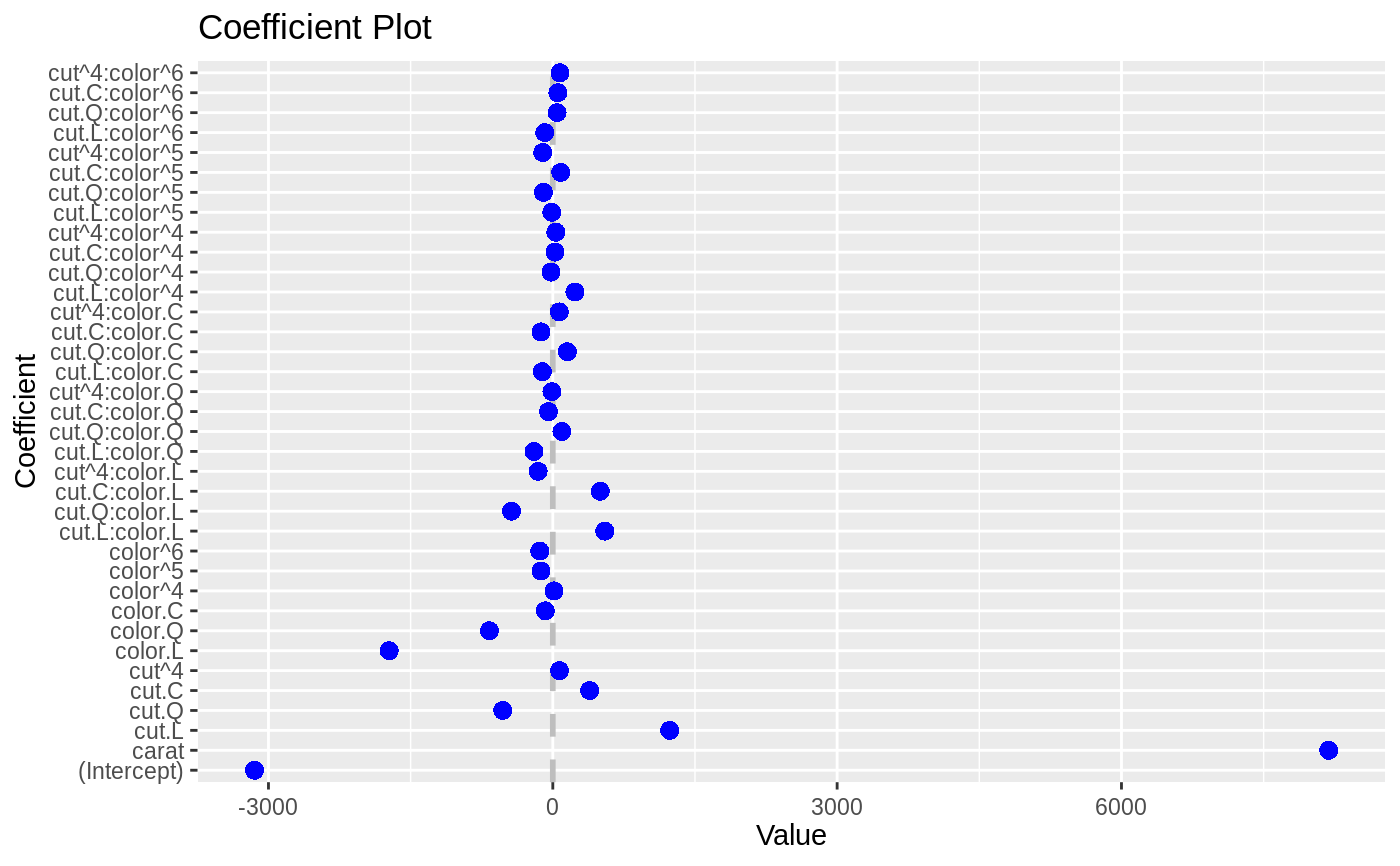
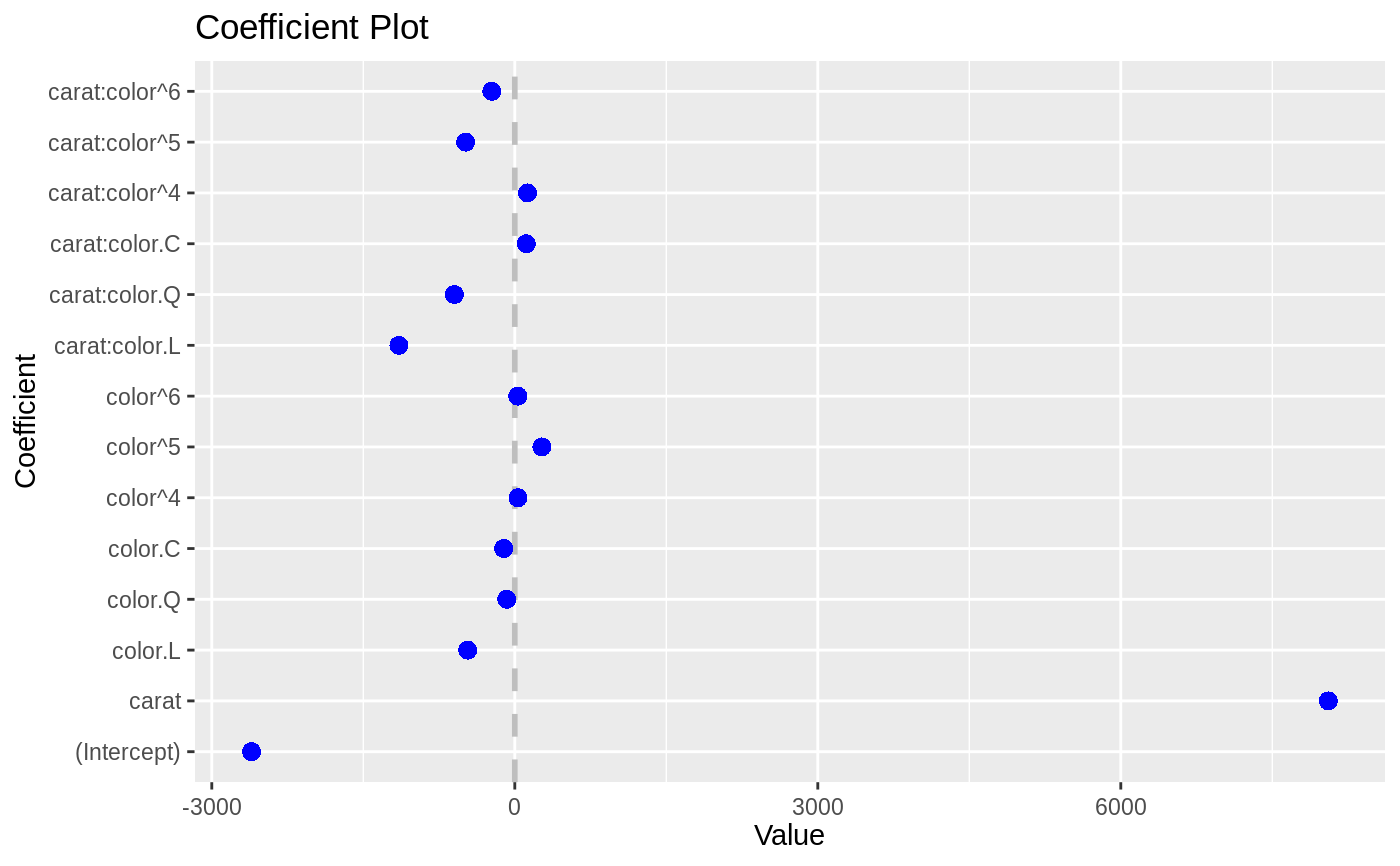
A graphical display of the coefficients and standard errors from a fitted model, this function uses a data.frame as the input.

Examples

data(diamonds)
head(diamonds)
#> # A tibble: 6 x 10
#>   carat cut       color clarity depth table price     x     y     z
#>   <dbl> <ord>     <ord> <ord>   <dbl> <dbl> <int> <dbl> <dbl> <dbl>
#> 1 0.23  Ideal     E     SI2      61.5    55   326  3.95  3.98  2.43
#> 2 0.21  Premium   E     SI1      59.8    61   326  3.89  3.84  2.31
#> 3 0.23  Good      E     VS1      56.9    65   327  4.05  4.07  2.31
#> 4 0.290 Premium   I     VS2      62.4    58   334  4.2   4.23  2.63
#> 5 0.31  Good      J     SI2      63.3    58   335  4.34  4.35  2.75
#> 6 0.24  Very Good J     VVS2     62.8    57   336  3.94  3.96  2.48
model1 <- lm(price ~ carat + cut*color, data=diamonds)
model2 <- lm(price ~ carat*color, data=diamonds)
df1 <- coefplot(model1, plot=FALSE)
df2 <- coefplot(model2, plot=FALSE)
coefplot(df1)
coefplot(df2)