fit a GLM with lasso or elasticnet regularization

Fit a generalized linear model via penalized maximum likelihood. The regularization path is computed for the lasso or elasticnet penalty at a grid of values for the regularization parameter lambda. Can deal with all shapes of data, including very large sparse data matrices. Fits linear, logistic and multinomial, poisson, and Cox regression models.

glmnet(x, y, family = c("gaussian", "binomial", "poisson", "multinomial",
  "cox", "mgaussian"), weights, offset = NULL, alpha = 1,
  nlambda = 100, lambda.min.ratio = ifelse(nobs < nvars, 0.01, 1e-04),
  lambda = NULL, standardize = TRUE, intercept = TRUE,
  thresh = 1e-07, dfmax = nvars + 1, pmax = min(dfmax * 2 + 20,
  nvars), exclude, penalty.factor = rep(1, nvars), lower.limits = -Inf,
  upper.limits = Inf, maxit = 1e+05, type.gaussian = ifelse(nvars <
  500, "covariance", "naive"), type.logistic = c("Newton",
  "modified.Newton"), standardize.response = FALSE,
  type.multinomial = c("ungrouped", "grouped"), relax = FALSE,
  trace.it = 0, ...)

relax.glmnet(fit, x, ..., maxp = n - 3, path = FALSE,
  check.args = TRUE)

Arguments

x	input matrix, of dimension nobs x nvars; each row is an observation vector. Can be in sparse matrix format (inherit from class "sparseMatrix" as in package Matrix; not yet available for family="cox")
y	response variable. Quantitative for family="gaussian", or family="poisson" (non-negative counts). For family="binomial" should be either a factor with two levels, or a two-column matrix of counts or proportions (the second column is treated as the target class; for a factor, the last level in alphabetical order is the target class). For family="multinomial", can be a nc>=2 level factor, or a matrix with nc columns of counts or proportions. For either "binomial" or "multinomial", if y is presented as a vector, it will be coerced into a factor. For family="cox", y should be a two-column matrix with columns named 'time' and 'status'. The latter is a binary variable, with '1' indicating death, and '0' indicating right censored. The function Surv() in package survival produces such a matrix. For family="mgaussian", y is a matrix of quantitative responses.
family	Response type (see above)
weights	observation weights. Can be total counts if responses are proportion matrices. Default is 1 for each observation
offset	A vector of length nobs that is included in the linear predictor (a nobs x nc matrix for the "multinomial" family). Useful for the "poisson" family (e.g. log of exposure time), or for refining a model by starting at a current fit. Default is NULL. If supplied, then values must also be supplied to the predict function.
alpha	The elasticnet mixing parameter, with \(0\le\alpha\le 1\). The penalty is defined as $$(1-\alpha)/2||\beta||_2^2+\alpha||\beta||_1.$$ alpha=1 is the lasso penalty, and alpha=0 the ridge penalty.
nlambda	The number of lambda values - default is 100.
lambda.min.ratio	Smallest value for lambda, as a fraction of lambda.max, the (data derived) entry value (i.e. the smallest value for which all coefficients are zero). The default depends on the sample size nobs relative to the number of variables nvars. If nobs > nvars, the default is 0.0001, close to zero. If nobs < nvars, the default is 0.01. A very small value of lambda.min.ratio will lead to a saturated fit in the nobs < nvars case. This is undefined for "binomial" and "multinomial" models, and glmnet will exit gracefully when the percentage deviance explained is almost 1.
lambda	A user supplied lambda sequence. Typical usage is to have the program compute its own lambda sequence based on nlambda and lambda.min.ratio. Supplying a value of lambda overrides this. WARNING: use with care. Avoid supplying a single value for lambda (for predictions after CV use predict() instead). Supply instead a decreasing sequence of lambda values. glmnet relies on its warms starts for speed, and its often faster to fit a whole path than compute a single fit.
standardize	Logical flag for x variable standardization, prior to fitting the model sequence. The coefficients are always returned on the original scale. Default is standardize=TRUE. If variables are in the same units already, you might not wish to standardize. See details below for y standardization with family="gaussian".
intercept	Should intercept(s) be fitted (default=TRUE) or set to zero (FALSE)
thresh	Convergence threshold for coordinate descent. Each inner coordinate-descent loop continues until the maximum change in the objective after any coefficient update is less than thresh times the null deviance. Defaults value is 1E-7.
dfmax	Limit the maximum number of variables in the model. Useful for very large nvars, if a partial path is desired.
pmax	Limit the maximum number of variables ever to be nonzero
exclude	Indices of variables to be excluded from the model. Default is none. Equivalent to an infinite penalty factor (next item).
penalty.factor	Separate penalty factors can be applied to each coefficient. This is a number that multiplies lambda to allow differential shrinkage. Can be 0 for some variables, which implies no shrinkage, and that variable is always included in the model. Default is 1 for all variables (and implicitly infinity for variables listed in exclude). Note: the penalty factors are internally rescaled to sum to nvars, and the lambda sequence will reflect this change.
lower.limits	Vector of lower limits for each coefficient; default -Inf. Each of these must be non-positive. Can be presented as a single value (which will then be replicated), else a vector of length nvars
upper.limits	Vector of upper limits for each coefficient; default Inf. See lower.limits
maxit	Maximum number of passes over the data for all lambda values; default is 10^5.
type.gaussian	Two algorithm types are supported for (only) family="gaussian". The default when nvar<500 is type.gaussian="covariance", and saves all inner-products ever computed. This can be much faster than type.gaussian="naive", which loops through nobs every time an inner-product is computed. The latter can be far more efficient for nvar >> nobs situations, or when nvar > 500.
type.logistic	If "Newton" then the exact hessian is used (default), while "modified.Newton" uses an upper-bound on the hessian, and can be faster.
standardize.response	This is for the family="mgaussian" family, and allows the user to standardize the response variables
type.multinomial	If "grouped" then a grouped lasso penalty is used on the multinomial coefficients for a variable. This ensures they are all in our out together. The default is "ungrouped"
relax	If TRUE then for each active set in the path of solutions, the model is refit without any regularization. See details for more information. This argument is new, and users may experience convergence issues with small datasets, especially with non-gaussian families. Limiting the value of 'maxp' can alleviate these issues in some cases.
trace.it	If trace.it=1, then a progress bar is displayed; useful for big models that take a long time to fit.
...	Additional argument used in relax.glmnet. These include some of the original arguments to 'glmnet', and each must be named if used.
fit	For relax.glmnet a fitted 'glmnet' object
maxp	a limit on how many relaxed coefficients are allowed. Default is 'n-3', where 'n' is the sample size. This may not be sufficient for non-gaussian familes, in which case users should supply a smaller value. This argument can be supplied directly to 'glmnet'.
path	Since glmnet does not do stepsize optimization, the Newton algorithm can get stuck and not converge, especially with relaxed fits. With path=TRUE, each relaxed fit on a particular set of variables is computed pathwise using the original sequence of lambda values (with a zero attached to the end). Not needed for Gaussian models, and should not be used unless needed, since will lead to longer compute times. Default is path=FALSE. appropriate subset of variables
check.args	Should relax.glmnet make sure that all the data dependent arguments used in creating 'fit' have been resupplied. Default is 'TRUE'.

Value

An object with S3 class "glmnet","*" , where "*" is "elnet", "lognet", "multnet", "fishnet" (poisson), "coxnet" or "mrelnet" for the various types of models. If the model was created with relax=TRUE then this class has a prefix class of "relaxed".

call

the call that produced this object

a0

Intercept sequence of length length(lambda)

beta

For "elnet", "lognet", "fishnet" and "coxnet" models, a nvars x length(lambda) matrix of coefficients, stored in sparse column format ("CsparseMatrix"). For "multnet" and "mgaussian", a list of nc such matrices, one for each class.

lambda

The actual sequence of lambda values used. When alpha=0, the largest lambda reported does not quite give the zero coefficients reported (lambda=inf would in principle). Instead, the largest lambda for alpha=0.001 is used, and the sequence of lambda values is derived from this.

dev.ratio

The fraction of (null) deviance explained (for "elnet", this is the R-square). The deviance calculations incorporate weights if present in the model. The deviance is defined to be 2*(loglike_sat - loglike), where loglike_sat is the log-likelihood for the saturated model (a model with a free parameter per observation). Hence dev.ratio=1-dev/nulldev.

nulldev

Null deviance (per observation). This is defined to be 2*(loglike_sat -loglike(Null)); The NULL model refers to the intercept model, except for the Cox, where it is the 0 model.

df

The number of nonzero coefficients for each value of lambda. For "multnet", this is the number of variables with a nonzero coefficient for any class.

dfmat

For "multnet" and "mrelnet" only. A matrix consisting of the number of nonzero coefficients per class

dim

dimension of coefficient matrix (ices)

nobs

number of observations

npasses

total passes over the data summed over all lambda values

offset

a logical variable indicating whether an offset was included in the model

jerr

error flag, for warnings and errors (largely for internal debugging).

relaxed

If relax=TRUE, this additional item is another glmnet object with different values for beta and dev.ratio

Details

The sequence of models implied by lambda is fit by coordinate descent. For family="gaussian" this is the lasso sequence if alpha=1, else it is the elasticnet sequence. For the other families, this is a lasso or elasticnet regularization path for fitting the generalized linear regression paths, by maximizing the appropriate penalized log-likelihood (partial likelihood for the "cox" model). Sometimes the sequence is truncated before nlambda values of lambda have been used, because of instabilities in the inverse link functions near a saturated fit. glmnet(...,family="binomial") fits a traditional logistic regression model for the log-odds. glmnet(...,family="multinomial") fits a symmetric multinomial model, where each class is represented by a linear model (on the log-scale). The penalties take care of redundancies. A two-class "multinomial" model will produce the same fit as the corresponding "binomial" model, except the pair of coefficient matrices will be equal in magnitude and opposite in sign, and half the "binomial" values. Note that the objective function for "gaussian" is $$1/2 RSS/nobs + \lambda*penalty,$$ and for the other models it is $$-loglik/nobs + \lambda*penalty.$$ Note also that for "gaussian", glmnet standardizes y to have unit variance (using 1/n rather than 1/(n-1) formula) before computing its lambda sequence (and then unstandardizes the resulting coefficients); if you wish to reproduce/compare results with other software, best to supply a standardized y. The coefficients for any predictor variables with zero variance are set to zero for all values of lambda. The latest two features in glmnet are the family="mgaussian" family and the type.multinomial="grouped" option for multinomial fitting. The former allows a multi-response gaussian model to be fit, using a "group -lasso" penalty on the coefficients for each variable. Tying the responses together like this is called "multi-task" learning in some domains. The grouped multinomial allows the same penalty for the family="multinomial" model, which is also multi-responsed. For both of these the penalty on the coefficient vector for variable j is $$(1-\alpha)/2||\beta_j||_2^2+\alpha||\beta_j||_2.$$ When alpha=1 this is a group-lasso penalty, and otherwise it mixes with quadratic just like elasticnet. A small detail in the Cox model: if death times are tied with censored times, we assume the censored times occurred just before the death times in computing the Breslow approximation; if users prefer the usual convention of after, they can add a small number to all censoring times to achieve this effect. If relax=TRUE a duplicate sequence of models is produced, where each active set in the elastic-net path is refit without regularization. The result of this is a matching "glmnet" object which is stored on the original object in a component named "relaxed", and is part of the glmnet output. Generally users will not call relax.glmnet directly, unless the original 'glmnet' object took a long time to fit. But if they do, they must supply the fit, and all the original arguments used to create that fit. They can limit the length of the relaxed path via 'maxp'.

References

Friedman, J., Hastie, T. and Tibshirani, R. (2008) Regularization Paths for Generalized Linear Models via Coordinate Descent, https://web.stanford.edu/~hastie/Papers/glmnet.pdf
Journal of Statistical Software, Vol. 33(1), 1-22 Feb 2010
https://www.jstatsoft.org/v33/i01/
Simon, N., Friedman, J., Hastie, T., Tibshirani, R. (2011) Regularization Paths for Cox's Proportional Hazards Model via Coordinate Descent, Journal of Statistical Software, Vol. 39(5) 1-13
https://www.jstatsoft.org/v39/i05/
Tibshirani, Robert, Bien, J., Friedman, J., Hastie, T.,Simon, N.,Taylor, J. and Tibshirani, Ryan. (2012) Strong Rules for Discarding Predictors in Lasso-type Problems, JRSSB vol 74,
https://statweb.stanford.edu/~tibs/ftp/strong.pdf
Stanford Statistics Technical Report
https://arxiv.org/abs/1707.08692
Hastie, T., Tibshirani, Robert, Tibshirani, Ryan (2019) Extended Comparisons of Best Subset Selection, Forward Stepwise Selection, and the Lasso
Glmnet Vignette https://web.stanford.edu/~hastie/glmnet/glmnet_alpha.html

See also

print, predict, coef and plot methods, and the cv.glmnet function.

Examples

# Gaussian
x = matrix(rnorm(100 * 20), 100, 20)
y = rnorm(100)
fit1 = glmnet(x, y)
print(fit1)
#> 
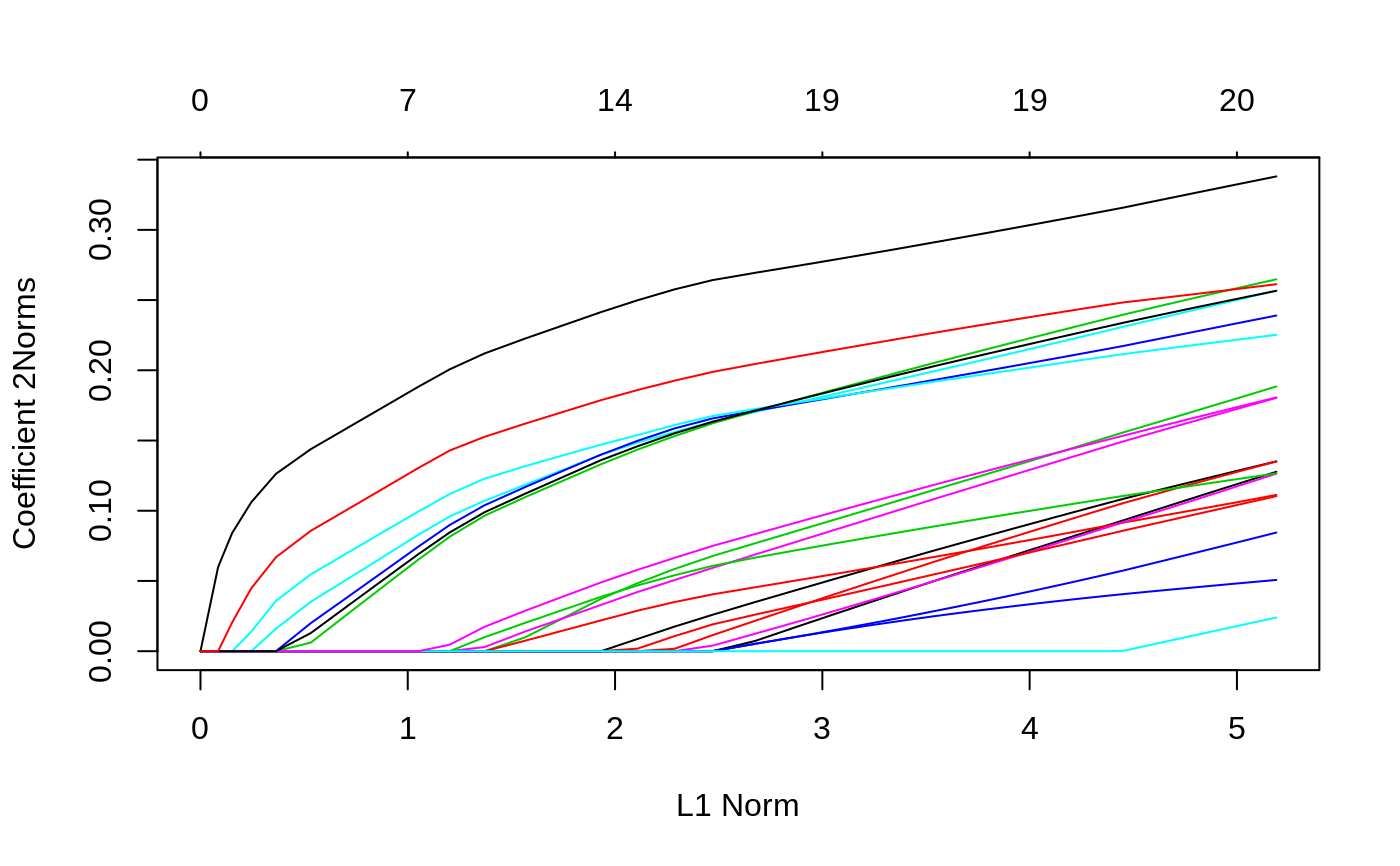
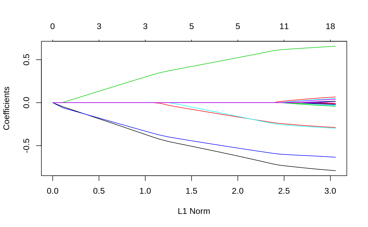
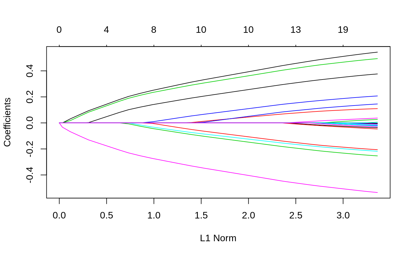
#> Call:  glmnet(x = x, y = y) 
#> 
#>    Df    %Dev   Lambda
#> 1   0 0.00000 0.241100
#> 2   1 0.01156 0.219700
#> 3   1 0.02115 0.200100
#> 4   1 0.02912 0.182400
#> 5   3 0.04378 0.166200
#> 6   4 0.06253 0.151400
#> 7   4 0.08111 0.137900
#> 8   5 0.09782 0.125700
#> 9   6 0.11390 0.114500
#> 10  6 0.12960 0.104400
#> 11  7 0.14280 0.095080
#> 12  7 0.15630 0.086640
#> 13  8 0.16780 0.078940
#> 14  9 0.17870 0.071930
#> 15 11 0.18950 0.065540
#> 16 12 0.19990 0.059720
#> 17 12 0.20880 0.054410
#> 18 12 0.21620 0.049580
#> 19 12 0.22240 0.045170
#> 20 13 0.22780 0.041160
#> 21 15 0.23360 0.037500
#> 22 15 0.23870 0.034170
#> 23 15 0.24300 0.031140
#> 24 17 0.24700 0.028370
#> 25 17 0.25070 0.025850
#> 26 18 0.25420 0.023550
#> 27 18 0.25710 0.021460
#> 28 18 0.25940 0.019550
#> 29 18 0.26140 0.017820
#> 30 18 0.26310 0.016230
#> 31 18 0.26440 0.014790
#> 32 19 0.26560 0.013480
#> 33 19 0.26660 0.012280
#> 34 19 0.26740 0.011190
#> 35 19 0.26810 0.010200
#> 36 19 0.26860 0.009290
#> 37 19 0.26910 0.008464
#> 38 19 0.26950 0.007713
#> 39 19 0.26980 0.007027
#> 40 19 0.27010 0.006403
#> 41 19 0.27030 0.005834
#> 42 19 0.27050 0.005316
#> 43 19 0.27060 0.004844
#> 44 19 0.27080 0.004413
#> 45 19 0.27090 0.004021
#> 46 19 0.27100 0.003664
#> 47 19 0.27100 0.003339
#> 48 19 0.27110 0.003042
#> 49 19 0.27110 0.002772
#> 50 19 0.27120 0.002525
#> 51 19 0.27120 0.002301
#> 52 19 0.27130 0.002097
#> 53 19 0.27130 0.001910
#> 54 19 0.27130 0.001741
#> 55 19 0.27130 0.001586
#> 56 19 0.27130 0.001445
#> 57 19 0.27130 0.001317
#> 58 19 0.27130 0.001200
#> 59 20 0.27140 0.001093
#> 60 20 0.27140 0.000996
#> 61 20 0.27140 0.000908
#> 62 20 0.27140 0.000827
#> 63 20 0.27140 0.000754
#> 64 20 0.27140 0.000687
#> 65 20 0.27140 0.000626
#> 66 20 0.27140 0.000570
coef(fit1, s = 0.01)  # extract coefficients at a single value of lambda
#> 21 x 1 sparse Matrix of class "dgCMatrix"
#>                        1
#> (Intercept)  0.121560872
#> V1           0.038296244
#> V2           .          
#> V3          -0.190479022
#> V4           0.064542607
#> V5          -0.004777782
#> V6           0.061976448
#> V7          -0.179189556
#> V8          -0.046220308
#> V9           0.034984779
#> V10         -0.106203233
#> V11          0.066413300
#> V12          0.243634220
#> V13         -0.055261320
#> V14          0.025203468
#> V15         -0.085658378
#> V16         -0.213164488
#> V17         -0.045210307
#> V18         -0.119723910
#> V19          0.162356337
#> V20         -0.030741349
predict(fit1, newx = x[1:10, ], s = c(0.01, 0.005))  # make predictions
#>                1          2
#>  [1,]  0.2118785  0.2176091
#>  [2,] -0.3985763 -0.4511024
#>  [3,]  0.2561177  0.2647228
#>  [4,] -0.5173629 -0.5419171
#>  [5,] -0.4270423 -0.4629741
#>  [6,] -0.1174245 -0.1194081
#>  [7,] -0.6621495 -0.6991950
#>  [8,]  0.2762641  0.2982341
#>  [9,]  0.8359337  0.8617435
#> [10,] -0.5872074 -0.6115066

# Relaxed
fit1r = glmnet(x, y, relax = TRUE)  # can be used with any model

# multivariate gaussian
y = matrix(rnorm(100 * 3), 100, 3)
fit1m = glmnet(x, y, family = "mgaussian")
plot(fit1m, type.coef = "2norm")

# binomial
g2 = sample(1:2, 100, replace = TRUE)
fit2 = glmnet(x, g2, family = "binomial")
fit2r = glmnet(x,g2, family = "binomial", relax=TRUE)
fit2rp = glmnet(x,g2, family = "binomial", relax=TRUE, path=TRUE)

# multinomial
g4 = sample(1:4, 100, replace = TRUE)
fit3 = glmnet(x, g4, family = "multinomial")
fit3a = glmnet(x, g4, family = "multinomial", type.multinomial = "grouped")
# poisson
N = 500
p = 20
nzc = 5
x = matrix(rnorm(N * p), N, p)
beta = rnorm(nzc)
f = x[, seq(nzc)] %*% beta
mu = exp(f)
y = rpois(N, mu)
fit = glmnet(x, y, family = "poisson")
plot(fit)
pfit = predict(fit, x, s = 0.001, type = "response")
plot(pfit, y)

# Cox
set.seed(10101)
N = 1000
p = 30
nzc = p/3
x = matrix(rnorm(N * p), N, p)
beta = rnorm(nzc)
fx = x[, seq(nzc)] %*% beta/3
hx = exp(fx)
ty = rexp(N, hx)
tcens = rbinom(n = N, prob = 0.3, size = 1)  # censoring indicator
y = cbind(time = ty, status = 1 - tcens)  # y=Surv(ty,1-tcens) with library(survival)
fit = glmnet(x, y, family = "cox")
plot(fit)

# Sparse
n = 10000
p = 200
nzc = trunc(p/10)
x = matrix(rnorm(n * p), n, p)
iz = sample(1:(n * p), size = n * p * 0.85, replace = FALSE)
x[iz] = 0
sx = Matrix(x, sparse = TRUE)
inherits(sx, "sparseMatrix")  #confirm that it is sparse
#> [1] TRUE
beta = rnorm(nzc)
fx = x[, seq(nzc)] %*% beta
eps = rnorm(n)
y = fx + eps
px = exp(fx)
px = px/(1 + px)
ly = rbinom(n = length(px), prob = px, size = 1)
system.time(fit1 <- glmnet(sx, y))
#>    user  system elapsed 
#>   0.299   0.000   0.298 
system.time(fit2n <- glmnet(x, y))
#>    user  system elapsed 
#>   0.257   0.008   0.265