Body Temperature Series of Beaver 1

Reynolds (1994) describes a small part of a study of the long-term temperature dynamics of beaver Castor canadensis in north-central Wisconsin. Body temperature was measured by telemetry every 10 minutes for four females, but data from a one period of less than a day for each of two animals is used there.

beav1

Format

The beav1 data frame has 114 rows and 4 columns. This data frame contains the following columns:

day: Day of observation (in days since the beginning of 1990), December 12--13.
time: Time of observation, in the form 0330 for 3.30am.
temp: Measured body temperature in degrees Celsius.
activ: Indicator of activity outside the retreat.

Note

The observation at 22:20 is missing.

Source

P. S. Reynolds (1994) Time-series analyses of beaver body temperatures. Chapter 11 of Lange, N., Ryan, L., Billard, L., Brillinger, D., Conquest, L. and Greenhouse, J. eds (1994) Case Studies in Biometry. New York: John Wiley and Sons.

References

Venables, W. N. and Ripley, B. D. (2002) Modern Applied Statistics with S. Fourth edition. Springer.

Examples

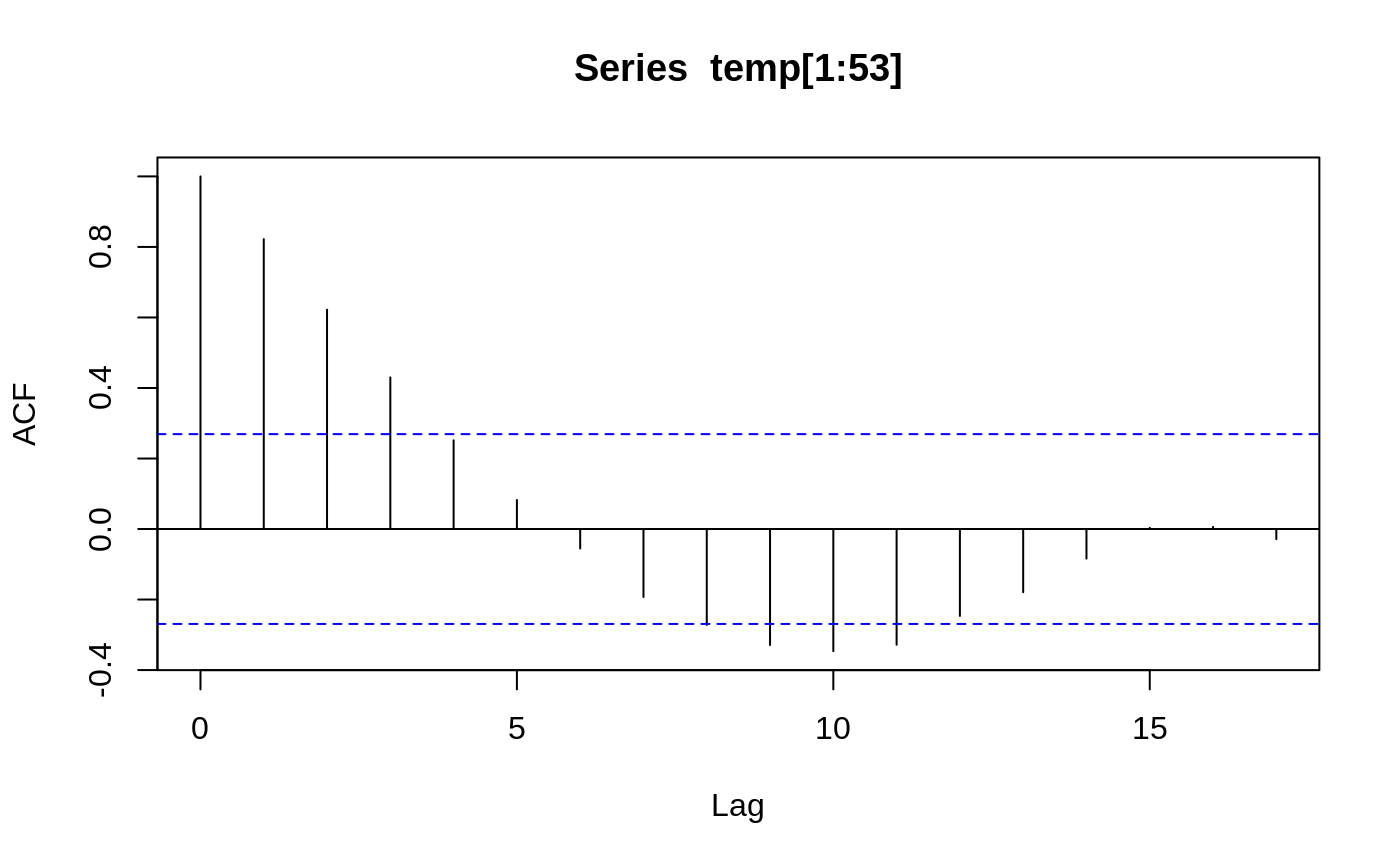
beav1 <- within(beav1,
               hours <- 24*(day-346) + trunc(time/100) + (time%%100)/60)
plot(beav1$hours, beav1$temp, type="l", xlab="time",
   ylab="temperature", main="Beaver 1")
usr <- par("usr"); usr[3:4] <- c(-0.2, 8); par(usr=usr)
lines(beav1$hours, beav1$activ, type="s", lty=2)
temp <- ts(c(beav1$temp[1:82], NA, beav1$temp[83:114]),
           start = 9.5, frequency = 6)
activ <- ts(c(beav1$activ[1:82], NA, beav1$activ[83:114]),
            start = 9.5, frequency = 6)

acf(temp[1:53])
acf(temp[1:53], type = "partial")
ar(temp[1:53])
#> 
#> Call:
#> ar(x = temp[1:53])
#> 
#> Coefficients:
#>      1  
#> 0.8222  
#> 
#> Order selected 1  sigma^2 estimated as  0.01011
act <- c(rep(0, 10), activ)
X <- cbind(1, act = act[11:125], act1 = act[10:124],
          act2 = act[9:123], act3 = act[8:122])
alpha <- 0.80
stemp <- as.vector(temp - alpha*lag(temp, -1))
sX <- X[-1, ] - alpha * X[-115,]
beav1.ls <- lm(stemp ~ -1 + sX, na.action = na.omit)
summary(beav1.ls, cor = FALSE)
#> 
#> Call:
#> lm(formula = stemp ~ -1 + sX, na.action = na.omit)
#> 
#> Residuals:
#>      Min       1Q   Median       3Q      Max 
#> -0.21317 -0.04317  0.00683  0.05483  0.37683 
#> 
#> Coefficients:
#>        Estimate Std. Error t value Pr(>|t|)    
#> sX     36.85587    0.03922 939.833  < 2e-16 ***
#> sXact   0.25400    0.03930   6.464 3.37e-09 ***
#> sXact1  0.17096    0.05100   3.352  0.00112 ** 
#> sXact2  0.16202    0.05147   3.148  0.00215 ** 
#> sXact3  0.10548    0.04310   2.448  0.01605 *  
#> ---
#> Signif. codes:  0 ‘***’ 0.001 ‘**’ 0.01 ‘*’ 0.05 ‘.’ 0.1 ‘ ’ 1
#> 
#> Residual standard error: 0.08096 on 104 degrees of freedom
#>   (5 observations deleted due to missingness)
#> Multiple R-squared:  0.9999,	Adjusted R-squared:  0.9999 
#> F-statistic: 1.81e+05 on 5 and 104 DF,  p-value: < 2.2e-16
#> 
rm(temp, activ)