Using .SD for Data Analysis
2019-12-31
Source:../../vignettes/datatable-sd-usage.Rmd
datatable-sd-usage.RmdThis vignette will explain the most common ways to use the .SD variable in your data.table analyses. It is an adaptation of this answer given on StackOverflow.
What is .SD?
In the broadest sense, .SD is just shorthand for capturing a variable that comes up frequently in the context of data analysis. It can be understood to stand for Subset, Selfsame, or Self-reference of the Data. That is, .SD is in its most basic guise a reflexive reference to the data.table itself – as we’ll see in examples below, this is particularly helpful for chaining together “queries” (extractions/subsets/etc using [). In particular, this also means that .SD is itself a data.table (with the caveat that it does not allow assignment with :=).
The simpler usage of .SD is for column subsetting (i.e., when .SDcols is specified); as this version is much more straightforward to understand, we’ll cover that first below. The interpretation of .SD in its second usage, grouping scenarios (i.e., when by = or keyby = is specified), is slightly different, conceptually (though at core it’s the same, since, after all, a non-grouped operation is an edge case of grouping with just one group).
Loading and Previewing Lahman Data
To give this a more real-world feel, rather than making up data, let’s load some data sets about baseball from the Lahman database. In typical R usage, we’d simply load these data sets from the Lahman R package; in this vignette, we’ve pre-downloaded them directly from the package’s GitHub page instead.
load('Teams.RData')
setDT(Teams)
Teams
#       yearID lgID teamID franchID divID Rank   G Ghome  W  L DivWin WCWin LgWin
#    1:   1871   NA    BS1      BNA  <NA>    3  31    NA 20 10   <NA>  <NA>     N
#    2:   1871   NA    CH1      CNA  <NA>    2  28    NA 19  9   <NA>  <NA>     N
#    3:   1871   NA    CL1      CFC  <NA>    8  29    NA 10 19   <NA>  <NA>     N
#    4:   1871   NA    FW1      KEK  <NA>    7  19    NA  7 12   <NA>  <NA>     N
#    5:   1871   NA    NY2      NNA  <NA>    5  33    NA 16 17   <NA>  <NA>     N
#   ---
# 2891:   2018   NL    SLN      STL     C    3 162    81 88 74      N     N     N
# 2892:   2018   AL    TBA      TBD     E    3 162    81 90 72      N     N     N
# 2893:   2018   AL    TEX      TEX     W    5 162    81 67 95      N     N     N
# 2894:   2018   AL    TOR      TOR     E    4 162    81 73 89      N     N     N
# 2895:   2018   NL    WAS      WSN     E    2 162    81 82 80      N     N     N
#       WSWin   R   AB    H X2B X3B  HR  BB   SO  SB CS HBP SF  RA  ER  ERA CG
#    1:  <NA> 401 1372  426  70  37   3  60   19  73 16  NA NA 303 109 3.55 22
#    2:  <NA> 302 1196  323  52  21  10  60   22  69 21  NA NA 241  77 2.76 25
#    3:  <NA> 249 1186  328  35  40   7  26   25  18  8  NA NA 341 116 4.11 23
#    4:  <NA> 137  746  178  19   8   2  33    9  16  4  NA NA 243  97 5.17 19
#    5:  <NA> 302 1404  403  43  21   1  33   15  46 15  NA NA 313 121 3.72 32
#   ---
# 2891:     N 759 5498 1369 248   9 205 525 1380  63 32  80 48 691 622 3.85  1
# 2892:     N 716 5475 1415 274  43 150 540 1388 128 51 101 50 646 602 3.74  0
# 2893:     N 737 5453 1308 266  24 194 555 1484  74 35  88 34 848 783 4.92  1
# 2894:     N 709 5477 1336 320  16 217 499 1387  47 30  58 37 832 772 4.85  0
# 2895:     N 771 5517 1402 284  25 191 631 1289 119 33  59 40 682 649 4.04  2
#       SHO SV IPouts   HA HRA BBA  SOA   E  DP    FP                    name
#    1:   1  3    828  367   2  42   23 243  24 0.834    Boston Red Stockings
#    2:   0  1    753  308   6  28   22 229  16 0.829 Chicago White Stockings
#    3:   0  0    762  346  13  53   34 234  15 0.818  Cleveland Forest Citys
#    4:   1  0    507  261   5  21   17 163   8 0.803    Fort Wayne Kekiongas
#    5:   1  0    879  373   7  42   22 235  14 0.840        New York Mutuals
#   ---
# 2891:   8 43   4366 1354 144 593 1337 133 151 0.978     St. Louis Cardinals
# 2892:  14 52   4345 1236 164 501 1421  85 136 0.986          Tampa Bay Rays
# 2893:   5 42   4293 1516 222 491 1121 120 168 0.980           Texas Rangers
# 2894:   3 39   4301 1476 208 551 1298 101 138 0.983       Toronto Blue Jays
# 2895:   7 40   4338 1320 198 487 1417  64 115 0.989    Washington Nationals
#                                park attendance BPF PPF teamIDBR teamIDlahman45
#    1:           South End Grounds I         NA 103  98      BOS            BS1
#    2:       Union Base-Ball Grounds         NA 104 102      CHI            CH1
#    3:  National Association Grounds         NA  96 100      CLE            CL1
#    4:                Hamilton Field         NA 101 107      KEK            FW1
#    5:      Union Grounds (Brooklyn)         NA  90  88      NYU            NY2
#   ---
# 2891:             Busch Stadium III    3403587  97  96      STL            SLN
# 2892:               Tropicana Field    1154973  97  97      TBR            TBA
# 2893: Rangers Ballpark in Arlington    2107107 112 113      TEX            TEX
# 2894:                 Rogers Centre    2325281  97  98      TOR            TOR
# 2895:                Nationals Park    2529604 106 105      WSN            MON
#       teamIDretro
#    1:         BS1
#    2:         CH1
#    3:         CL1
#    4:         FW1
#    5:         NY2
#   ---
# 2891:         SLN
# 2892:         TBA
# 2893:         TEX
# 2894:         TOR
# 2895:         WAS

load('Pitching.RData')
setDT(Pitching)
Pitching
#         playerID yearID stint teamID lgID  W  L  G GS CG SHO SV IPouts   H  ER
#     1: bechtge01   1871     1    PH1   NA  1  2  3  3  2   0  0     78  43  23
#     2: brainas01   1871     1    WS3   NA 12 15 30 30 30   0  0    792 361 132
#     3: fergubo01   1871     1    NY2   NA  0  0  1  0  0   0  0      3   8   3
#     4: fishech01   1871     1    RC1   NA  4 16 24 24 22   1  0    639 295 103
#     5: fleetfr01   1871     1    NY2   NA  0  1  1  1  1   0  0     27  20  10
#    ---
# 46695: zamorda01   2018     1    NYN   NL  1  0 16  0  0   0  0     27   6   3
# 46696: zastrro01   2018     1    CHN   NL  1  0  6  0  0   0  0     17   6   3
# 46697: zieglbr01   2018     1    MIA   NL  1  5 53  0  0   0 10    156  49  23
# 46698: zieglbr01   2018     2    ARI   NL  1  1 29  0  0   0  0     65  22   9
# 46699: zimmejo02   2018     1    DET   AL  7  8 25 25  0   0  0    394 140  66
#        HR BB  SO BAOpp   ERA IBB WP HBP BK  BFP GF   R SH SF GIDP
#     1:  0 11   1    NA  7.96  NA  7  NA  0  146  0  42 NA NA   NA
#     2:  4 37  13    NA  4.50  NA  7  NA  0 1291  0 292 NA NA   NA
#     3:  0  0   0    NA 27.00  NA  2  NA  0   14  0   9 NA NA   NA
#     4:  3 31  15    NA  4.35  NA 20  NA  0 1080  1 257 NA NA   NA
#     5:  0  3   0    NA 10.00  NA  0  NA  0   57  0  21 NA NA   NA
#    ---
# 46695:  1  3  16 0.194  3.00   1  0   1  0   36  4   3  1  0    1
# 46696:  0  4   3 0.286  4.76   0  0   1  0   26  2   3  0  0    0
# 46697:  7 17  37 0.254  3.98   4  1   2  0  213 23  25  0  1   11
# 46698:  1  8  13 0.265  3.74   2  0   0  0   92  1   9  0  1    3
# 46699: 28 26 111 0.269  4.52   0  1   2  0  556  0  76  2  5    4
Readers up on baseball lingo should find the tables’ contents familiar; Teams records some statistics for a given team in a given year, while Pitching records statistics for a given pitcher in a given year. Please do check out the documentation and explore the data yourself a bit before proceeding to familiarize yourself with their structure.
.SD on Ungrouped Data
To illustrate what I mean about the reflexive nature of .SD, consider its most banal usage:
Pitching[ , .SD]
#         playerID yearID stint teamID lgID  W  L  G GS CG SHO SV IPouts   H  ER
#     1: bechtge01   1871     1    PH1   NA  1  2  3  3  2   0  0     78  43  23
#     2: brainas01   1871     1    WS3   NA 12 15 30 30 30   0  0    792 361 132
#     3: fergubo01   1871     1    NY2   NA  0  0  1  0  0   0  0      3   8   3
#     4: fishech01   1871     1    RC1   NA  4 16 24 24 22   1  0    639 295 103
#     5: fleetfr01   1871     1    NY2   NA  0  1  1  1  1   0  0     27  20  10
#    ---
# 46695: zamorda01   2018     1    NYN   NL  1  0 16  0  0   0  0     27   6   3
# 46696: zastrro01   2018     1    CHN   NL  1  0  6  0  0   0  0     17   6   3
# 46697: zieglbr01   2018     1    MIA   NL  1  5 53  0  0   0 10    156  49  23
# 46698: zieglbr01   2018     2    ARI   NL  1  1 29  0  0   0  0     65  22   9
# 46699: zimmejo02   2018     1    DET   AL  7  8 25 25  0   0  0    394 140  66
#        HR BB  SO BAOpp   ERA IBB WP HBP BK  BFP GF   R SH SF GIDP
#     1:  0 11   1    NA  7.96  NA  7  NA  0  146  0  42 NA NA   NA
#     2:  4 37  13    NA  4.50  NA  7  NA  0 1291  0 292 NA NA   NA
#     3:  0  0   0    NA 27.00  NA  2  NA  0   14  0   9 NA NA   NA
#     4:  3 31  15    NA  4.35  NA 20  NA  0 1080  1 257 NA NA   NA
#     5:  0  3   0    NA 10.00  NA  0  NA  0   57  0  21 NA NA   NA
#    ---
# 46695:  1  3  16 0.194  3.00   1  0   1  0   36  4   3  1  0    1
# 46696:  0  4   3 0.286  4.76   0  0   1  0   26  2   3  0  0    0
# 46697:  7 17  37 0.254  3.98   4  1   2  0  213 23  25  0  1   11
# 46698:  1  8  13 0.265  3.74   2  0   0  0   92  1   9  0  1    3
# 46699: 28 26 111 0.269  4.52   0  1   2  0  556  0  76  2  5    4
That is, Pitching[ , .SD] has simply returned the whole table, i.e., this was an overly verbose way of writing Pitching or Pitching[]:
In terms of subsetting, .SD is still a subset of the data, it’s just a trivial one (the set itself).
Column Subsetting: .SDcols
The first way to impact what .SD is is to limit the columns contained in .SD using the .SDcols argument to [:
# W: Wins; L: Losses; G: Games
Pitching[ , .SD, .SDcols = c('W', 'L', 'G')]
#         W  L  G
#     1:  1  2  3
#     2: 12 15 30
#     3:  0  0  1
#     4:  4 16 24
#     5:  0  1  1
#    ---
# 46695:  1  0 16
# 46696:  1  0  6
# 46697:  1  5 53
# 46698:  1  1 29
# 46699:  7  8 25
This is just for illustration and was pretty boring. But even this simply usage lends itself to a wide variety of highly beneficial / ubiquitous data manipulation operations:
Column Type Conversion
Column type conversion is a fact of life for data munging. Though fwrite recently gained the ability to declare the class of each column up front, not all data sets come from fread (e.g. in this vignette) and conversions back and forth among character/factor/numeric types are common. We can use .SD and .SDcols to batch-convert groups of columns to a common type.
We notice that the following columns are stored as character in the Teams data set, but might more logically be stored as factors:
# teamIDBR: Team ID used by Baseball Reference website
# teamIDlahman45: Team ID used in Lahman database version 4.5
# teamIDretro: Team ID used by Retrosheet
fkt = c('teamIDBR', 'teamIDlahman45', 'teamIDretro')
# confirm that they're stored as `character`
Teams[ , sapply(.SD, is.character), .SDcols = fkt]
#       teamIDBR teamIDlahman45    teamIDretro
#           TRUE           TRUE           TRUE
If you’re confused by the use of sapply here, note that it’s quite similar for base R data.frames:
setDF(Teams) # convert to data.frame for illustration
sapply(Teams[ , fkt], is.character)
#       teamIDBR teamIDlahman45    teamIDretro
#           TRUE           TRUE           TRUE
setDT(Teams) # convert back to data.table
The key to understanding this syntax is to recall that a data.table (as well as a data.frame) can be considered as a list where each element is a column – thus, sapply/lapply applies the FUN argument (in this case, is.character) to each column and returns the result as sapply/lapply usually would.
The syntax to now convert these columns to factor is very similar – simply add the := assignment operator:
Teams[ , (fkt) := lapply(.SD, factor), .SDcols = fkt]
# print out the first column to demonstrate success
head(unique(Teams[[fkt[1L]]]))
# [1] BOS CHI CLE KEK NYU ATH
# 101 Levels: ALT ANA ARI ATH ATL BAL BLA BLN BLU BOS BRA BRG BRO BSN BTT ... WSN
Note that we must wrap fkt in parentheses () to force data.table to interpret this as column names, instead of trying to assign a column named 'fkt'.
Actually, the .SDcols argument is quite flexible; above, we supplied a character vector of column names. In other situations, it is more convenient to supply an integer vector of column positions or a logical vector dictating include/exclude for each column. .SDcols even accepts regular expression-based pattern matching.
For example, we could do the following to convert all factor columns to character:
# while .SDcols accepts a logical vector,
#   := does not, so we need to convert to column
#   positions with which()
fkt_idx = which(sapply(Teams, is.factor))
Teams[ , (fkt_idx) := lapply(.SD, as.character), .SDcols = fkt_idx]
head(unique(Teams[[fkt_idx[1L]]]))
# [1] "NA" "NL" "AA" "UA" "PL" "AL"
Lastly, we can do pattern-based matching of columns in .SDcols to select all columns which contain team back to factor:
Teams[ , .SD, .SDcols = patterns('team')]
#       teamID teamIDBR teamIDlahman45 teamIDretro
#    1:    BS1      BOS            BS1         BS1
#    2:    CH1      CHI            CH1         CH1
#    3:    CL1      CLE            CL1         CL1
#    4:    FW1      KEK            FW1         FW1
#    5:    NY2      NYU            NY2         NY2
#   ---
# 2891:    SLN      STL            SLN         SLN
# 2892:    TBA      TBR            TBA         TBA
# 2893:    TEX      TEX            TEX         TEX
# 2894:    TOR      TOR            TOR         TOR
# 2895:    WAS      WSN            MON         WAS

# now convert these columns to factor;
#   value = TRUE in grep() is for the LHS of := to
#   get column names instead of positions
team_idx = grep('team', names(Teams), value = TRUE)
Teams[ , (team_idx) := lapply(.SD, factor), .SDcols = team_idx]
** A proviso to the above: explicitly using column numbers (like DT[ , (1) := rnorm(.N)]) is bad practice and can lead to silently corrupted code over time if column positions change. Even implicitly using numbers can be dangerous if we don’t keep smart/strict control over the ordering of when we create the numbered index and when we use it.
Controlling a Model’s Right-Hand Side
Varying model specification is a core feature of robust statistical analysis. Let’s try and predict a pitcher’s ERA (Earned Runs Average, a measure of performance) using the small set of covariates available in the Pitching table. How does the (linear) relationship between W (wins) and ERA vary depending on which other covariates are included in the specification?
Here’s a short script leveraging the power of .SD which explores this question:
# this generates a list of the 2^k possible extra variables
#   for models of the form ERA ~ G + (...)
extra_var = c('yearID', 'teamID', 'G', 'L')
models = unlist(
  lapply(0L:length(extra_var), combn, x = extra_var, simplify = FALSE),
  recursive = FALSE
)

# here are 16 visually distinct colors, taken from the list of 20 here:
#   https://sashat.me/2017/01/11/list-of-20-simple-distinct-colors/
col16 = c('#e6194b', '#3cb44b', '#ffe119', '#0082c8',
          '#f58231', '#911eb4', '#46f0f0', '#f032e6',
          '#d2f53c', '#fabebe', '#008080', '#e6beff',
          '#aa6e28', '#fffac8', '#800000', '#aaffc3')

par(oma = c(2, 0, 0, 0))
lm_coef = sapply(models, function(rhs) {
  # using ERA ~ . and data = .SD, then varying which
  #   columns are included in .SD allows us to perform this
  #   iteration over 16 models succinctly.
  #   coef(.)['W'] extracts the W coefficient from each model fit
  Pitching[ , coef(lm(ERA ~ ., data = .SD))['W'], .SDcols = c('W', rhs)]
})
barplot(lm_coef, names.arg = sapply(models, paste, collapse = '/'),
        main = 'Wins Coefficient\nWith Various Covariates',
        col = col16, las = 2L, cex.names = .8)
The coefficient always has the expected sign (better pitchers tend to have more wins and fewer runs allowed), but the magnitude can vary substantially depending on what else we control for.
Conditional Joins
data.table syntax is beautiful for its simplicity and robustness. The syntax x[i] flexibly handles three common approaches to subsetting – when i is a logical vector, x[i] will return those rows of x corresponding to where i is TRUE; when i is another data.table (or a list), a (right) join is performed (in the plain form, using the keys of x and i, otherwise, when on = is specified, using matches of those columns); and when i is a character, it is interpreted as shorthand for x[list(i)], i.e., as a join.
This is great in general, but falls short when we wish to perform a conditional join, wherein the exact nature of the relationship among tables depends on some characteristics of the rows in one or more columns.
This example is admittedly a tad contrived, but illustrates the idea; see here (1, 2) for more.
The goal is to add a column team_performance to the Pitching table that records the team’s performance (rank) of the best pitcher on each team (as measured by the lowest ERA, among pitchers with at least 6 recorded games).
# to exclude pitchers with exceptional performance in a few games,
#   subset first; then define rank of pitchers within their team each year
#   (in general, we should put more care into the 'ties.method' of frank)
Pitching[G > 5, rank_in_team := frank(ERA), by = .(teamID, yearID)]
Pitching[rank_in_team == 1, team_performance :=
           Teams[.SD, Rank, on = c('teamID', 'yearID')]]
Note that the x[y] syntax returns nrow(y) values (i.e., it’s a right join), which is why .SD is on the right in Teams[.SD] (since the RHS of := in this case requires nrow(Pitching[rank_in_team == 1]) values.
Grouped .SD operations
Often, we’d like to perform some operation on our data at the group level. When we specify by = (or keyby =), the mental model for what happens when data.table processes j is to think of your data.table as being split into many component sub-data.tables, each of which corresponds to a single value of your by variable(s):
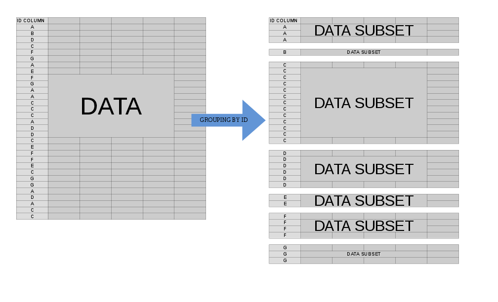
Grouping, Illustrated
In the case of grouping, .SD is multiple in nature – it refers to each of these sub-data.tables, one-at-a-time (slightly more accurately, the scope of .SD is a single sub-data.table). This allows us to concisely express an operation that we’d like to perform on each sub-data.table before the re-assembled result is returned to us.
This is useful in a variety of settings, the most common of which are presented here:
Group Subsetting
Let’s get the most recent season of data for each team in the Lahman data. This can be done quite simply with:
# the data is already sorted by year; if it weren't
#   we could do Teams[order(yearID), .SD[.N], by = teamID]
Teams[ , .SD[.N], by = teamID]
#      teamID yearID lgID franchID divID Rank   G Ghome  W  L DivWin WCWin LgWin
#   1:    BS1   1875   NA      BNA  <NA>    1  82    NA 71  8   <NA>  <NA>     Y
#   2:    CH1   1871   NA      CNA  <NA>    2  28    NA 19  9   <NA>  <NA>     N
#   3:    CL1   1872   NA      CFC  <NA>    7  22    NA  6 16   <NA>  <NA>     N
#   4:    FW1   1871   NA      KEK  <NA>    7  19    NA  7 12   <NA>  <NA>     N
#   5:    NY2   1875   NA      NNA  <NA>    6  71    NA 30 38   <NA>  <NA>     N
#  ---
# 145:    ANA   2004   AL      ANA     W    1 162    81 92 70      Y     N     N
# 146:    ARI   2018   NL      ARI     W    3 162    81 82 80      N     N     N
# 147:    MIL   2018   NL      MIL     C    1 163    81 96 67      Y     N     N
# 148:    TBA   2018   AL      TBD     E    3 162    81 90 72      N     N     N
# 149:    MIA   2018   NL      FLA     E    5 161    81 63 98      N     N     N
#      WSWin   R   AB    H X2B X3B  HR  BB   SO  SB CS HBP SF  RA  ER  ERA CG SHO
#   1:  <NA> 831 3515 1128 167  51  15  33   52  93 37  NA NA 343 152 1.87 60  10
#   2:  <NA> 302 1196  323  52  21  10  60   22  69 21  NA NA 241  77 2.76 25   0
#   3:  <NA> 174  943  272  28   5   0  17   13  12  3  NA NA 254 126 5.70 15   0
#   4:  <NA> 137  746  178  19   8   2  33    9  16  4  NA NA 243  97 5.17 19   1
#   5:  <NA> 328 2685  633  82  21   7  19   47  20 24  NA NA 425 174 2.46 70   3
#  ---
# 145:     N 836 5675 1603 272  37 162 450  942 143 46  73 41 734 692 4.28  2  11
# 146:     N 693 5460 1283 259  50 176 560 1460  79 25  52 45 644 605 3.72  2   9
# 147:     N 754 5542 1398 252  24 218 537 1458 124 32  58 41 659 606 3.73  0  14
# 148:     N 716 5475 1415 274  43 150 540 1388 128 51 101 50 646 602 3.74  0  14
# 149:     N 589 5488 1303 222  24 128 455 1384  45 31  73 31 809 762 4.76  1  12
#      SV IPouts   HA HRA BBA  SOA   E  DP    FP                    name
#   1: 17   2196  751   2  33  110 483  56 0.870    Boston Red Stockings
#   2:  1    753  308   6  28   22 229  16 0.829 Chicago White Stockings
#   3:  0    597  285   6  24   11 184  17 0.816  Cleveland Forest Citys
#   4:  0    507  261   5  21   17 163   8 0.803    Fort Wayne Kekiongas
#   5:  0   1910  718   4  21   77 526  30 0.838        New York Mutuals
#  ---
# 145: 50   4363 1476 170 502 1164  90 126 0.985          Anaheim Angels
# 146: 39   4389 1313 174 522 1448  75 152 0.988    Arizona Diamondbacks
# 147: 49   4383 1259 173 553 1428 108 141 0.982       Milwaukee Brewers
# 148: 52   4345 1236 164 501 1421  85 136 0.986          Tampa Bay Rays
# 149: 30   4326 1388 192 605 1249  83 133 0.986           Miami Marlins
#                              park attendance BPF PPF teamIDBR teamIDlahman45
#   1:          South End Grounds I         NA 103  96      BOS            BS1
#   2:      Union Base-Ball Grounds         NA 104 102      CHI            CH1
#   3: National Association Grounds         NA  96 100      CLE            CL1
#   4:               Hamilton Field         NA 101 107      KEK            FW1
#   5:     Union Grounds (Brooklyn)         NA  99 100      NYU            NY2
#  ---
# 145:    Angels Stadium of Anaheim    3375677  97  97      ANA            ANA
# 146:                  Chase Field    2242695 108 107      ARI            ARI
# 147:                  Miller Park    2850875 102 101      MIL            ML4
# 148:              Tropicana Field    1154973  97  97      TBR            TBA
# 149:                 Marlins Park     811104  89  90      MIA            FLO
#      teamIDretro
#   1:         BS1
#   2:         CH1
#   3:         CL1
#   4:         FW1
#   5:         NY2
#  ---
# 145:         ANA
# 146:         ARI
# 147:         MIL
# 148:         TBA
# 149:         MIA
Recall that .SD is itself a data.table, and that .N refers to the total number of rows in a group (it’s equal to nrow(.SD) within each group), so .SD[.N] returns the entirety of .SD for the final row associated with each teamID.
Another common version of this is to use .SD[1L] instead to get the first observation for each group, or .SD[sample(.N, 1L)] to return a random row for each group.
Group Optima
Suppose we wanted to return the best year for each team, as measured by their total number of runs scored (R; we could easily adjust this to refer to other metrics, of course). Instead of taking a fixed element from each sub-data.table, we now define the desired index dynamically as follows:
Teams[ , .SD[which.max(R)], by = teamID]
#      teamID yearID lgID franchID divID Rank   G Ghome   W  L DivWin WCWin LgWin
#   1:    BS1   1875   NA      BNA  <NA>    1  82    NA  71  8   <NA>  <NA>     Y
#   2:    CH1   1871   NA      CNA  <NA>    2  28    NA  19  9   <NA>  <NA>     N
#   3:    CL1   1871   NA      CFC  <NA>    8  29    NA  10 19   <NA>  <NA>     N
#   4:    FW1   1871   NA      KEK  <NA>    7  19    NA   7 12   <NA>  <NA>     N
#   5:    NY2   1872   NA      NNA  <NA>    3  56    NA  34 20   <NA>  <NA>     N
#  ---
# 145:    ANA   2000   AL      ANA     W    3 162    81  82 80      N     N     N
# 146:    ARI   1999   NL      ARI     W    1 162    81 100 62      Y     N     N
# 147:    MIL   1999   NL      MIL     C    5 161    80  74 87      N     N     N
# 148:    TBA   2009   AL      TBD     E    3 162    81  84 78      N     N     N
# 149:    MIA   2017   NL      FLA     E    2 162    78  77 85      N     N     N
#      WSWin   R   AB    H X2B X3B  HR  BB   SO  SB CS HBP SF  RA  ER  ERA CG SHO
#   1:  <NA> 831 3515 1128 167  51  15  33   52  93 37  NA NA 343 152 1.87 60  10
#   2:  <NA> 302 1196  323  52  21  10  60   22  69 21  NA NA 241  77 2.76 25   0
#   3:  <NA> 249 1186  328  35  40   7  26   25  18  8  NA NA 341 116 4.11 23   0
#   4:  <NA> 137  746  178  19   8   2  33    9  16  4  NA NA 243  97 5.17 19   1
#   5:  <NA> 523 2426  670  87  14   4  58   52  59 22  NA NA 362 172 3.02 54   3
#  ---
# 145:     N 864 5628 1574 309  34 236 608 1024  93 52  47 43 869 805 5.00  5   3
# 146:     N 908 5658 1566 289  46 216 588 1045 137 39  48 60 676 615 3.77 16   9
# 147:     N 815 5582 1524 299  30 165 658 1065  81 33  55 51 886 813 5.07  2   5
# 148:     N 803 5462 1434 297  36 199 642 1229 194 61  49 45 754 686 4.33  3   5
# 149:     N 778 5602 1497 271  31 194 486 1282  91 30  67 41 822 772 4.82  1   7
#      SV IPouts   HA HRA BBA  SOA   E  DP    FP                    name
#   1: 17   2196  751   2  33  110 483  56 0.870    Boston Red Stockings
#   2:  1    753  308   6  28   22 229  16 0.829 Chicago White Stockings
#   3:  0    762  346  13  53   34 234  15 0.818  Cleveland Forest Citys
#   4:  0    507  261   5  21   17 163   8 0.803    Fort Wayne Kekiongas
#   5:  1   1536  622   2  33   46 323  33 0.868        New York Mutuals
#  ---
# 145: 46   4344 1534 228 662  846 134 182 0.978          Anaheim Angels
# 146: 42   4402 1387 176 543 1198 104 132 0.983    Arizona Diamondbacks
# 147: 40   4328 1618 213 616  987 127 146 0.979       Milwaukee Brewers
# 148: 41   4282 1421 183 515 1125  98 135 0.983          Tampa Bay Rays
# 149: 34   4328 1450 193 627 1202  73 156 0.988           Miami Marlins
#                              park attendance BPF PPF teamIDBR teamIDlahman45
#   1:          South End Grounds I         NA 103  96      BOS            BS1
#   2:      Union Base-Ball Grounds         NA 104 102      CHI            CH1
#   3: National Association Grounds         NA  96 100      CLE            CL1
#   4:               Hamilton Field         NA 101 107      KEK            FW1
#   5:     Union Grounds (Brooklyn)         NA  93  92      NYU            NY2
#  ---
# 145:   Edison International Field    2066982 102 103      ANA            ANA
# 146:            Bank One Ballpark    3019654 101 101      ARI            ARI
# 147:               County Stadium    1701796  99  99      MIL            ML4
# 148:              Tropicana Field    1874962  98  97      TBR            TBA
# 149:                 Marlins Park    1583014  93  93      MIA            FLO
#      teamIDretro
#   1:         BS1
#   2:         CH1
#   3:         CL1
#   4:         FW1
#   5:         NY2
#  ---
# 145:         ANA
# 146:         ARI
# 147:         MIL
# 148:         TBA
# 149:         MIA
Note that this approach can of course be combined with .SDcols to return only portions of the data.table for each .SD (with the caveat that .SDcols should be fixed across the various subsets)
NB: .SD[1L] is currently optimized by GForce (see also), data.table internals which massively speed up the most common grouped operations like sum or mean – see ?GForce for more details and keep an eye on/voice support for feature improvement requests for updates on this front: 1, 2, 3, 4, 5, 6
Grouped Regression
Returning to the inquiry above regarding the relationship between ERA and W, suppose we expect this relationship to differ by team (i.e., there’s a different slope for each team). We can easily re-run this regression to explore the heterogeneity in this relationship as follows (noting that the standard errors from this approach are generally incorrect – the specification ERA ~ W*teamID will be better – this approach is easier to read and the coefficients are OK):
# Overall coefficient for comparison
overall_coef = Pitching[ , coef(lm(ERA ~ W))['W']]
# use the .N > 20 filter to exclude teams with few observations
Pitching[ , if (.N > 20L) .(w_coef = coef(lm(ERA ~ W))['W']), by = teamID
          ][ , hist(w_coef, 20L, las = 1L,
                    xlab = 'Fitted Coefficient on W',
                    ylab = 'Number of Teams', col = 'darkgreen',
                    main = 'Team-Level Distribution\nWin Coefficients on ERA')]
abline(v = overall_coef, lty = 2L, col = 'red')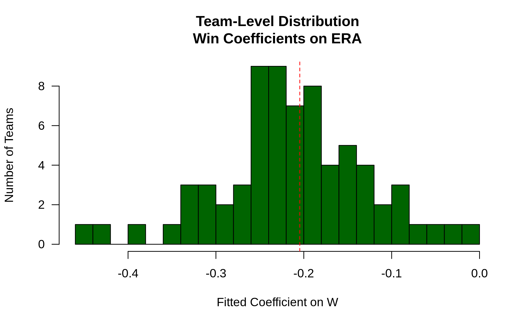
While there is indeed a fair amount of heterogeneity, there’s a distinct concentration around the observed overall value.
The above is just a short introduction of the power of .SD in facilitating beautiful, efficient code in data.table!