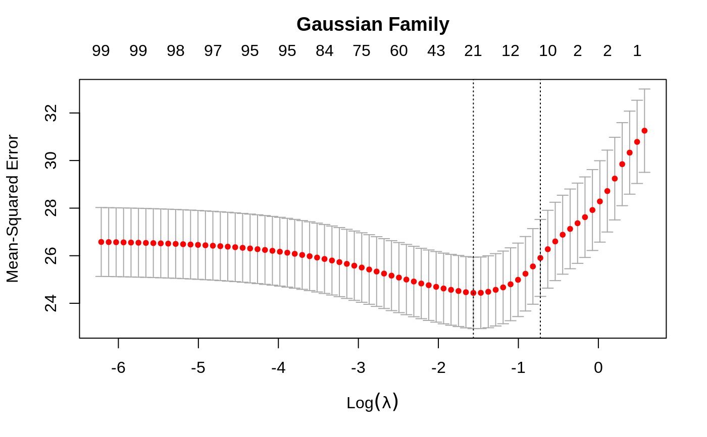
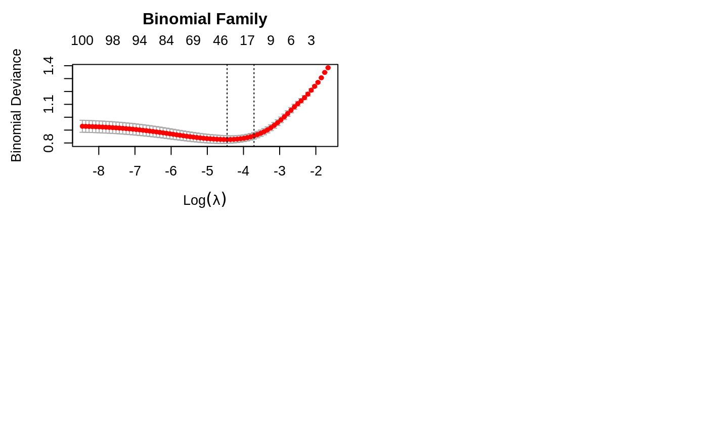
plot the cross-validation curve produced by cv.glmnet

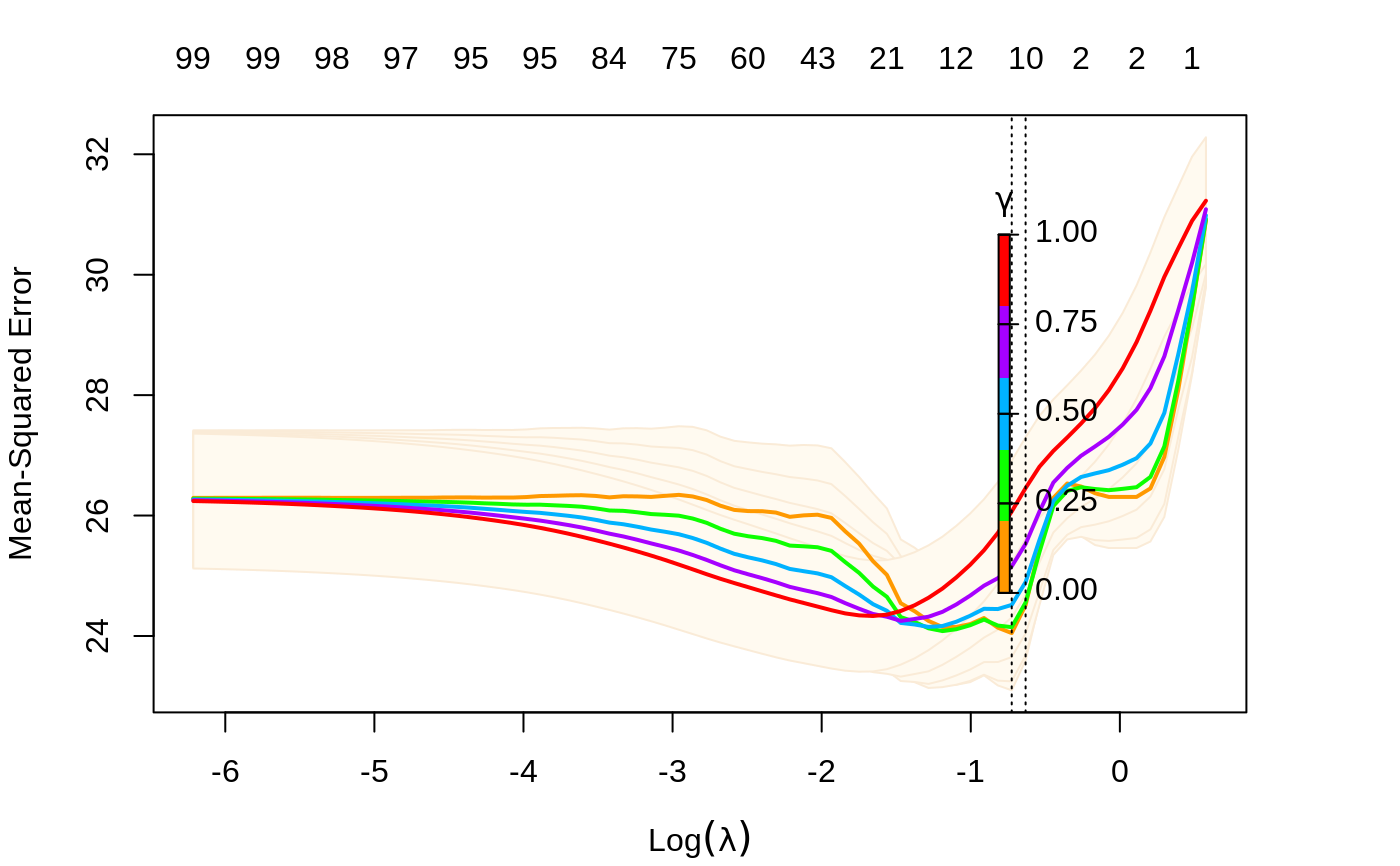
Plots the cross-validation curve, and upper and lower standard deviation curves, as a function of the lambda values used. If the object has class "cv.relaxed" a different plot is produced, showing both lambda and gamma

# S3 method for cv.glmnet
plot(x, sign.lambda = 1, ...)

# S3 method for cv.relaxed
plot(x, se.bands = TRUE, ...)

Arguments

x	fitted "cv.glmnet" object
sign.lambda	Either plot against log(lambda) (default) or its negative if sign.lambda=-1.
...	Other graphical parameters to plot
se.bands	Should shading be produced to show standard-error bands; default is TRUE

Details

A plot is produced, and nothing is returned.

References

Friedman, J., Hastie, T. and Tibshirani, R. (2008) Regularization Paths for Generalized Linear Models via Coordinate Descent

See also

glmnet and cv.glmnet.

Examples

set.seed(1010)
n = 1000
p = 100
nzc = trunc(p/10)
x = matrix(rnorm(n * p), n, p)
beta = rnorm(nzc)
fx = (x[, seq(nzc)] %*% beta)
eps = rnorm(n) * 5
y = drop(fx + eps)
px = exp(fx)
px = px/(1 + px)
ly = rbinom(n = length(px), prob = px, size = 1)
cvob1 = cv.glmnet(x, y)
plot(cvob1)
title("Gaussian Family", line = 2.5)
cvob1r = cv.glmnet(x, y, relax = TRUE)
plot(cvob1r)
frame()
set.seed(1011)
par(mfrow = c(2, 2), mar = c(4.5, 4.5, 4, 1))
cvob2 = cv.glmnet(x, ly, family = "binomial")
plot(cvob2)
title("Binomial Family", line = 2.5)
## set.seed(1011)
## cvob3 = cv.glmnet(x, ly, family = "binomial", type = "class")
## plot(cvob3)
## title("Binomial Family", line = 2.5)