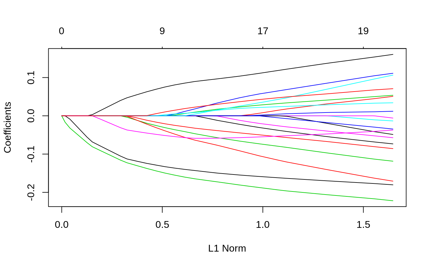
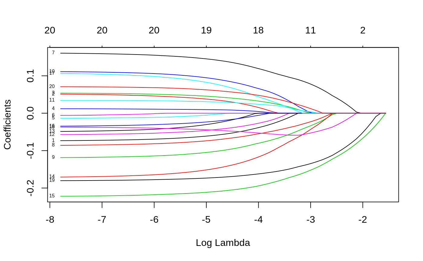
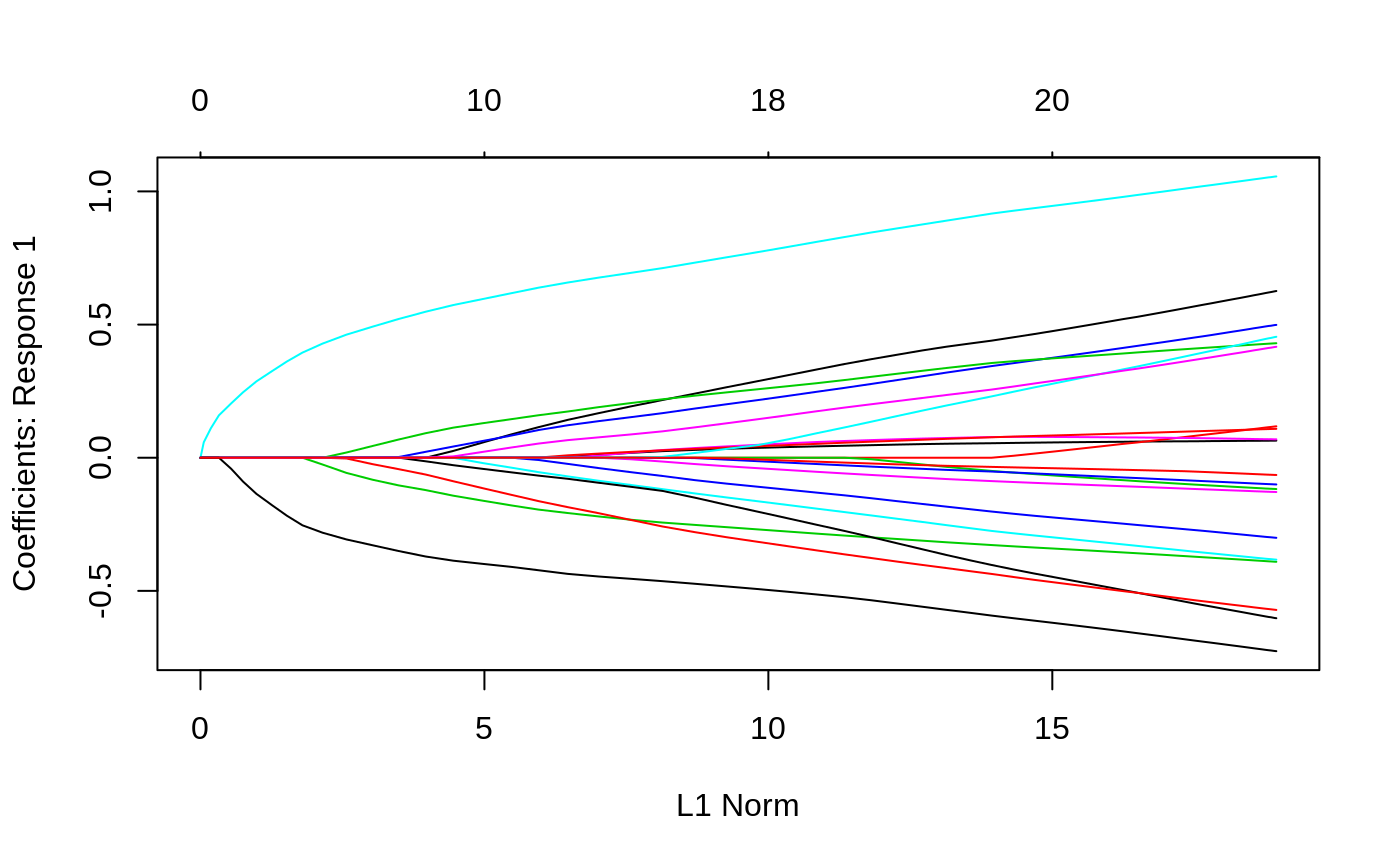
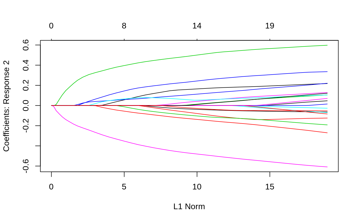
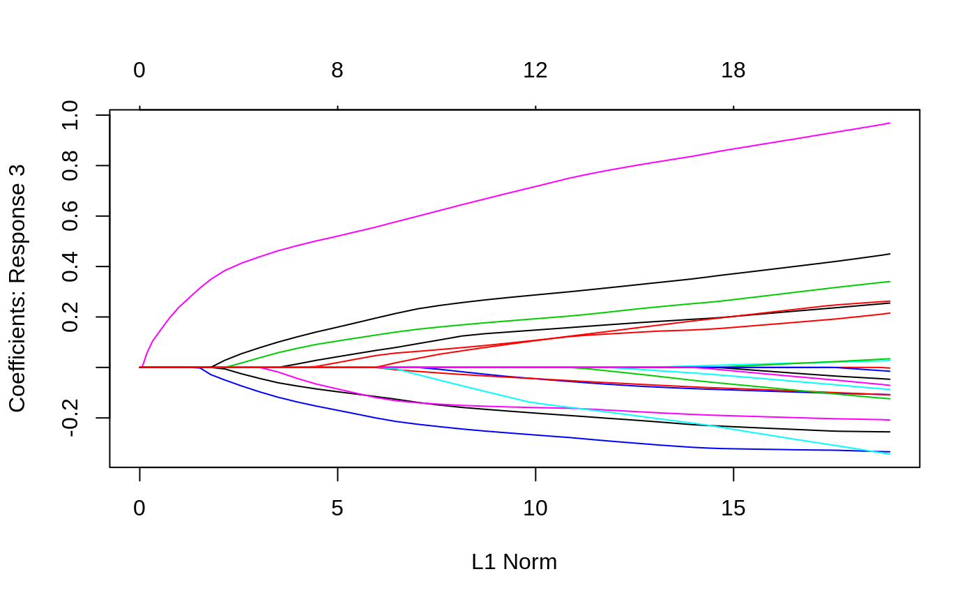
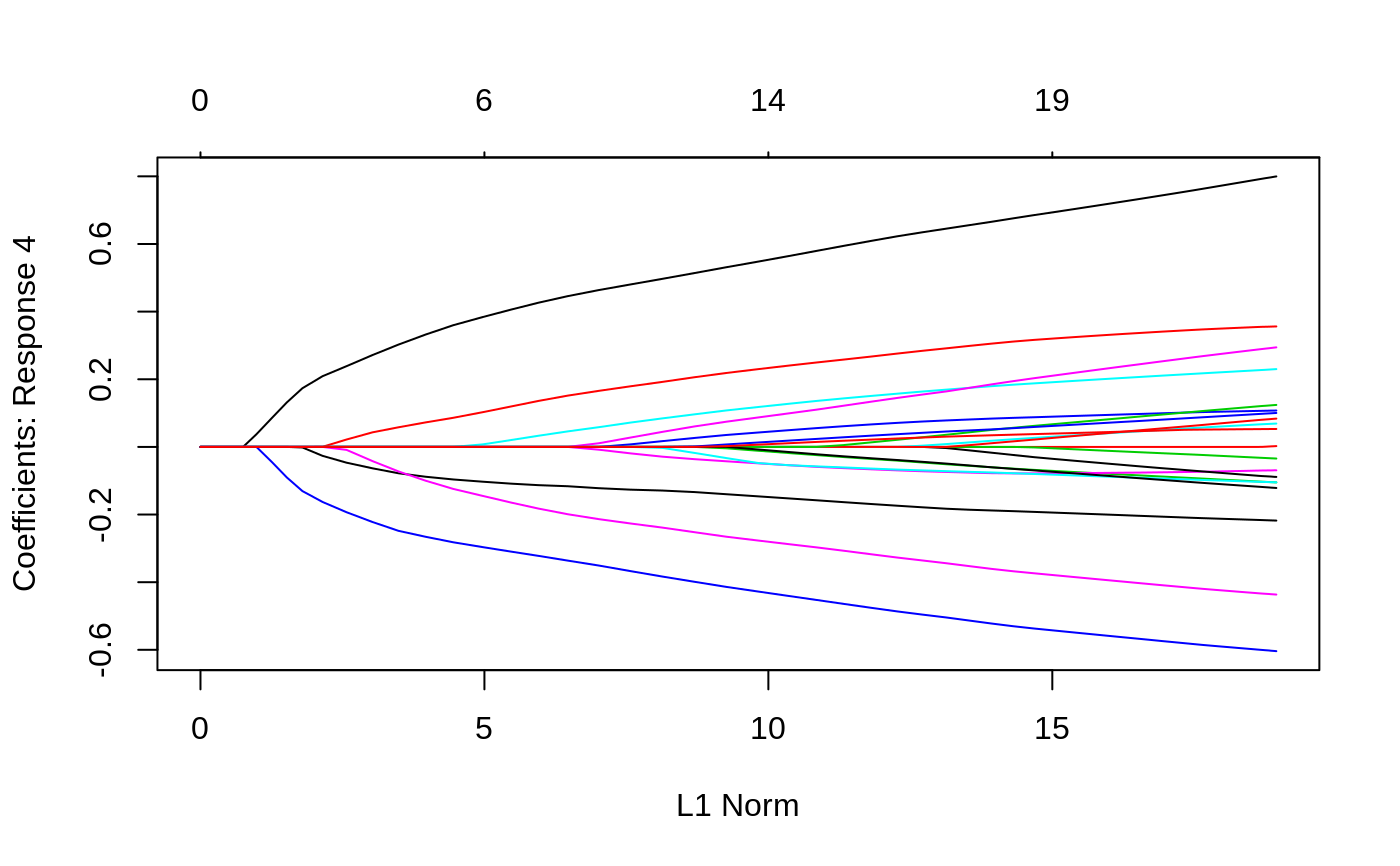
plot coefficients from a "glmnet" object

Produces a coefficient profile plot of the coefficient paths for a fitted "glmnet" object.

# S3 method for glmnet
plot(x, xvar = c("norm", "lambda", "dev"),
  label = FALSE, ...)

# S3 method for mrelnet
plot(x, xvar = c("norm", "lambda", "dev"),
  label = FALSE, type.coef = c("coef", "2norm"), ...)

# S3 method for multnet
plot(x, xvar = c("norm", "lambda", "dev"),
  label = FALSE, type.coef = c("coef", "2norm"), ...)

# S3 method for relaxed
plot(x, xvar = c("lambda", "dev"), label = FALSE,
  gamma = 1, ...)

Arguments

x	fitted "glmnet" model
xvar	What is on the X-axis. "norm" plots against the L1-norm of the coefficients, "lambda" against the log-lambda sequence, and "dev" against the percent deviance explained.
label	If TRUE, label the curves with variable sequence numbers.
...	Other graphical parameters to plot
type.coef	If type.coef="2norm" then a single curve per variable, else if type.coef="coef", a coefficient plot per response
gamma	Value of the mixing parameter for a "relaxed" fit

Details

A coefficient profile plot is produced. If x is a multinomial model, a coefficient plot is produced for each class.

References

Friedman, J., Hastie, T. and Tibshirani, R. (2008) Regularization Paths for Generalized Linear Models via Coordinate Descent

See also

glmnet, and print, predict and coef methods.

Examples

x=matrix(rnorm(100*20),100,20)
y=rnorm(100)
g2=sample(1:2,100,replace=TRUE)
g4=sample(1:4,100,replace=TRUE)
fit1=glmnet(x,y)
plot(fit1)
plot(fit1,xvar="lambda",label=TRUE)
fit3=glmnet(x,g4,family="multinomial")
plot(fit3,pch=19)